3 Constructs and Latent Variables in Psychometrics
3.1 The Importance of Psychometrics
Psychometrics, a field within psychology, focuses on quantifying and measuring mental attributes, behaviors, performance, and emotions. Despite significant advancements in psychometric modeling over the past centuries, its integration into conventional psychological testing remains limited. This is very concerning, given that measurement problems abound in human research (Cronbach & Meehl, 1955; Messick, 1989; Borsboom et. al., 2004). Scholars argue that applying psychometric models to formalize psychological theory holds promise for addressing these challenges (Borsboom, 2006). However, many psychologists continue to rely on traditional psychometric methods, such as internal consistency coefficients and principal component analyses, without much deviation from past practices. Consequently, the interpretation of psychological test scores often lacks rigor, highlighting the disconnect between psychometrics and psychology (Borsboom, 2006).
3.2 Misunderstandings in Psychometric Practice
Misunderstandings are prevalent in the field of psychometrics. For instance, many studies delve into the structure of individual differences using latent variable theory but employ Principal Component Analysis (PCA) for data analysis. However, PCA does not align with latent variable theory. Thus, extracting a principal component structure alone does not shed light on its correspondence with a supposed latent variable structure. PCA serves as a data reduction technique (Bartholomew, 2004), which, in itself, isn’t problematic as long as interpretations remain confined to principal components, which are essentially weighted sum scores.
Another example is the interpretation of group differences through observed scores. The interpretation of differences between groups regarding psychological attributes depends on measurement invariance (or measurement equivalence) between the groups being compared. There are several psychometric models and associated techniques to gain some control over this problem (Mellenbergh, 1989; Meredith, 1993; Millsap & Everson, 1993). However, almost no one cares about this, whether in Brazil or abroad, people simply evaluate the observed scores — without testing the invariance of the measurement models that relate these scores to psychological attributes. If you look at, for example, some of the most influential studies on group differences in intelligence, you rarely see invariance analyses. Consider for example the work of Herrnstein and Murray (1994) and Lynn and Vanhanen (2002). They infer differences in intelligence levels between groups from observed differences in IQ (by race and nationality) without even having performed a single test for invariance.
3.3 Obstacles to the Psychometric Revolution
Borsboom (2006) highlights a significant issue with psychometric models: they often challenge commonly accepted assumptions, such as measurement invariance. This leads researchers into fundamental questions about the structure of the phenomena they study and its relationship to observable data. Developing theories in this context is no simple task, potentially placing researchers in complex situations. Despite the importance of these inquiries in any scientific field, they aren’t widely embraced in psychology. Consequently, even if researchers can provide compelling models for their observations, publishing such results proves challenging, as many journal editors and reviewers lack familiarity with psychometric models. Additionally, the perceived complexity of psychometrics exacerbates this issue. Compounding matters are the prevailing research standards in psychology, which demand that scientific articles remain accessible, despite the inherently intricate nature of the subject matter – human behavior and its underlying mental processes.
3.4 The Artistry of Measuring the Mind
As defended by Maraun and Peters (2005), in scientific research, concepts are essential tools for identifying and organizing phenomena. Scientific outputs—such as observations, hypotheses, and theories—are expressed through language, which relies on concepts. These concepts are human creations, distinct from natural reality, and their correct usage is governed by linguistic rules. In the natural sciences, technical concepts are developed specifically for scientific purposes. These linguistic rules are so important as a means of scientific inquiry that can affect the reproducibility of scientific results (Schmalz et al., 2024). Although concepts are linguistic constructs, some describe features of the natural world, allowing scientists to discuss these realities accurately. The meaning of a concept is not “discovered” in the way scientific facts are, but rather established by human-defined rules of use. Science creates these rules but discovers the actual entities the term describes. Thus, while science aims to explain the natural world, it must also ensure that concepts are used correctly to convey those explanations (Maraun & Peters, 2005).
Psychologists investigate a wide range of these concepts that are crucial to understanding and improving everyday life. For instance, the study of stress and its impact on health helps to develop strategies for stress management that enhance well-being (Tetrick & Winslow, 2015). Another example comes from educational psychology, leading to improved educational methods that benefit students of all ages (Harackiewicz & Priniski, 2018) To study such phenomena, the history of psychology led to developments in the quantification of the human mind by measuring it (Michell, 2014). Measurement, as a fundamental scientific method, provides a means to determine, with varying degrees of validity and reliability, the level of an attribute present in the object or objects being studied. The reliability of these measurements can vary based on the precision of the tools and methods used, but the core purpose remains the same: to assess the extent of a particular attribute in a systematic and reproducible manner (Michell, 2001).
Seen by some as a fundamental liability (Trendler, 2013), measurement is based on constructs in many areas of psychological research, particularly in the study of individual differences. A construct is defined as “a conceptual system that refers to a set of entities—the construct referents—that are regarded as meaningfully related in some ways or for some purpose although they actually never occur all at once and that are therefore considered only on more abstract levels as a joint entity” (Uher, 2022, p. 14). A construct is a concept that has three characteristics (Cronbach & Meehl, 1955): (i) it is not defined by a single observable referent (for example, 1 item on a scale); (ii) cannot be observed directly; and (iii) its observable referents are not fully inclusive.
Constructs are not physical entities; rather, they are conceptual tools devised to efficiently represent specific sets of referents (Uher, 2023). However, there is a common tendency to confuse constructs with the actual phenomena they represent. This confusion, known as construct–referent conflation (Maraun & Gabriel, 2013), leads to the erroneous practice of mistaking scientific constructs—the tools of investigation—for the actual phenomena being studied (Uher, 2023). This criticism has repeatedly been made about psychological measures, with the conflation of IQ measures and the interpretation of what intelligence is as a very well-known example (Stanovich, 2009).
A similar issue arises with the item variables researchers use to encode and analyze information about study phenomena—the referents of these variables (e.g., an individual’s attitudes, behaviors, or beliefs) are often interpreted as though they themselves were the phenomena under study. This variable–referent conflation occurs when both the phenomena being studied (which reside within the subjects) and the item variables (which exist in data sets and are analyzed statistically) are labeled as ‘variables’ (Uher, 2021). Failing to clearly differentiate between the phenomena under investigation and the methods used to study them leads to the conflation of distinct scientific activities, complicating the task of distinguishing between them and ultimately distorting scientific concepts and procedures (Uher, 2022, 2023).
A latent variable is one (but not the only) statistical tool for studying constructs, and is commonly used in statistical analyzes to evaluate the relationship between constructs and their indicators (Spearman, 1904). A construct is operationally defined in terms of a number of items or indirect indicators, which are taken as an empirical analogue of a construct (Edwards & Bagozzi, 2000). These indicators are also called observed variables, which can be items in a self-report measure, interview, observations, or other means (DeVellis, 1991; Lord & Novick, 1968; Messick, 1995).
The reflective approach to latent variables is used by most methods in psychometrics that deal with measurement issues, often used in areas such as personality (John, 2021), well-being (Diener et al., 2010), criminology (Pechorro et al ., 2021), and others. The reflective approach is based on several assumptions, one of which is critical to its validity. It postulates a causal relationship between the latent variable and its indicators. This means that the variance and covariance in the indicators are dependent on changes in the latent variable (Bollen, 1989).
3.5 Ways to Represent a Construct
Usually, when running an Exploratory of Confirmatory Factor Analysis, we use the common factor model. This model sees the covariance between observable variables as a reflection of the influence of one or more factors and also a variance that is not explained. This would be different from network analysis, which allows covariance between items to have a cause between them. In other words, the psychometric model of factor analysis generally believes that item covariance occurs only because there is a latent factor that explains it. This is a very important assumption to keep in mind, as perhaps your construct does not fit the common factor model, but rather a network analysis. I will explain with an example given by Borsboom and Cramer (2013).
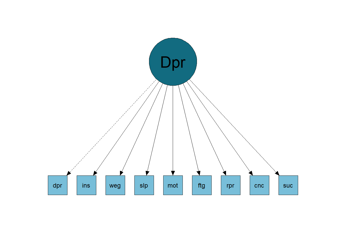
Below, we see the common factor model (Figure 3.1) of an instrument that measures major depression. In it, items measure aspects such as: feeling depressed, insomnia, weight gain, motor problems, fatigue, concentration problems, etc. We see from the image that the variation in scores on the items has a common cause, depression (that is, the higher the person’s level of depression, the more they report having these symptoms).
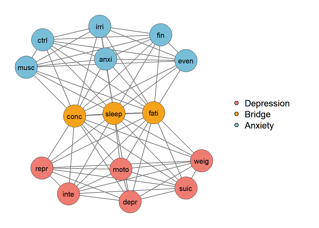
However, we can think that some items have relationships with each other that are not just due to depression. An example of this is the cause of concentration problems and its relationship with other symptoms. People who have problems sleeping become fatigued and, therefore, have problems concentrating (problems sleeping → fatigue → concentration problems). In other words, it is possible to infer a causal relationship between one observable variable and another, which breaks with the common factorial model assumption of local independence. A possible representation of this model is in the image below (Figure 3.2), where the items have causal relationships with each other.
So how do I know if my construct follows the common factor model or is more like network analysis? Well, often by theory! I know that researchers for a long time only cared about statistics to guide everything, but it is important for us to think about our constructs theoretically again and then test the theory empirically.
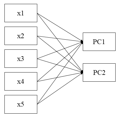
We have other types of models, like formative models. Formative models are usually analyzed using Principal Component Analysis, where the latent variables are formed by the manifest variables (or items). An example of a variable in the formative model is socioeconomic level, which can be explained by items such as income, place of residence, education, etc. Thus, this latent variable is a representation of the items. An example of a formative model can be seen in Figure 3.3.
Another model we have is the latent profile/classes model. It’s a reflective model like the Common Factor Model (i.e., factor analysis model, Item Response Theory models, etc.). However, the difference lies in the representation of the latent variable. While in the Common Factor Model the latent variable (such as Subjective Well-Being) is considered a continuous variable, in Latent Classes or Latent Profile models they are considered as categorical. The distinction between numerical representation between variables are given in Chapter 4.
3.6 The Platonic Relationship of Cause and Effect in Psychological Measures
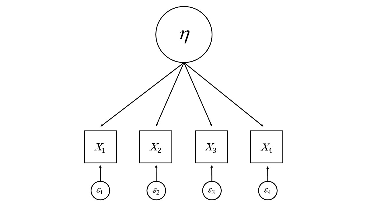
The validity of psychometric models depends on the validity of the causal assumptions they make, which are generally implicit to the user. Psychological tests (e.g., self-report questionnaires) are typically constructed to measure constructs, while the responses observed in such tests are believed to reflect the latent variable underlying them (Van Bork et al., 2017). For example, a person’s self-esteem is not observed directly, but we assume that it can be measured through items on an instrument. This line of thinking is the basis of the reflective approach, as represented by Figure 3.4. The reflective approach is applied to most psychometric models, such as classical test theory (Lord & Novick, 1968), the common factor model (Bartholomew, 1995; Speaman, 1904), item response theory models (Hambleton et al. al., 1991), latent class and latent profile analysis (B. O. Muthén & L. K. Muthén, 2000; Obersky, 2016), mixture models (Loken & Molenaar, 2008), latent growth models (Meredith & Tisak, 1990), reliability (Nunnally, 1978) and others, all crucial aspects of instrument development and evaluation.
Causal language is common across a wide range of research areas (Pearl, 2009) and has permeated the definition of reflective measures in psychometric literature. For example, measurement error is often characterized as part of an observed variable that is not “explained” by the construct (or true score; Lord & Novick, 1968; Nunnally, 1978). Furthermore, other authors clearly state the direction of causality from the construct to its indicators (DeVellis, 1991; Long, 1983). However, some authors defend the descriptivist (or formative) approach, which understands latent variables as a parsimonious summary of the data and not the underlying cause of the indicators (Jonas & Markon, 2016; Van Bork et al., 2017). The difference between the causal and descriptive approaches is that the first can be seen as a representation of a real-world phenomenon, while the second does not include a conceptual interpretation and only describes statistical dependencies between indicators (Moneta & Russo, 2014; Van Bork and others, 2017). Causal interpretation is important in many settings (Van Bork et al., 2017): (1) in research, establishing causal relationships is often aligned with the primary goal of explaining correlations between multiple indicators, rather than just summarizing them. them.; (2) a causal interpretation of the construct legitimizes the reflective approach and its shared variance rather than other models that take into account the unique variance of indicators, such as the network model (Borsboom & Cramer, 2013); (3) the causal interpretation resonates with the assumption of local independence (i.e., covariation between indicators disappears when conditioned on their common cause).
However, the simple use of causal language does not necessarily imply that the variables actually have causal relationships, this is an empirical question. To incorporate causality, one must adhere to the principles of causality from the philosophy of science within the psychological, social, and behavioral literature (Asher, 1983; Bagozzi, 1980; Bollen, 1989; Cook & Campbell, 1979; Heise, 1975; James et al. al., 1982).
Reflective measurement models, widely used in psychometrics, assume that latent variables cause linear changes in observable indicators, but this assumption is rarely validated (Bartholomew, 1995). In 1904, Spearman demonstrated that when a single latent factor is the cause of four or more observed variables, the difference in the products of certain pairs of covariances (or correlations) among these variables must equal zero. These relationships became known as “vanishing tetrads.” Spearman’s work, later explored in more depth by Bollen (1989) and Glymour et al. (2014), revealed that the correlation matrix of observed variables can show evidence of a common latent cause. Specifically, a common latent cause imposes constraints on the correlation matrix, allowing researchers to show evidence whether the data was generated by such a common cause (Bollen & Ting, 1993). This will be explained in depth in the next paragraphs.
3.7 Vanishing Tetrads
Linear models are usually meant to have a causal interpretation (Glymour & Scheines, 1986). Many linear models can be thought of as a directed graph that explicitly gives the causal relations. To understand the vanishing tetrads, consider a path from vertex \(u\) to vertex \(v\) in a directed graph to be a sequence of directed edges \(u → u2→ ...→ v\), with all arrows running in the same direction. Also, consider that a trek between \(u\) and \(v\) to be either a path from \(v\) to \(u\), or a path from \(u\) to \(v\), or a pair of paths from some vertex \(w\) to \(u\) and to \(v\) such that no more than one vertex occurs in both paths, or an undirected or bidirected arrow connecting \(u\) and \(v\).
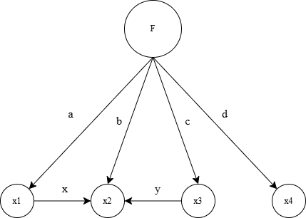
Consider the example from Glymour and Scheines (1986). In Figure 3.5, we have three treks between \(x1\) and \(x3\). The first trek is a direct edge from \(x3\) to \(x2\), with label \(y\). The second is a common cause from the latent variable \(F\), with labels \(b\) and \(c\). The last one is a common cause from \(F\) through variable \(x1\), with labels \(a\) and \(x\) on the path from \(F\) through \(x1\) to \(x2\), and label \(c\) on the path to \(x3\) directly from \(F\).
Formally, we say that any vertex \(u\) is into vertex \(w\) in a directed graph if and only if there is a directed edge (a single headed arrow such as \(→\)) from \(u\) to \(w\) (\(u → w\)). The rules for determining the structural equations and statistical constraints from the graph are as follows: (1) Each variable \(v\) in the graph is a linear functional of all of the variables that are into \(v\). (2) If there is no trek between variables \(u\) and \(v\), then \(u\) and \(v\) are statistically independent. (3) Variables connected by an undirected or double headed arrow (such as \(↔\)) are not assumed to be statistically independent. In effect, a double headed or undirected arrow signifies a covariance that receives no causal explanation in the model.
Representing causal models as directed graphs allows us to easily compute which tetrad equations a model implies. Any trek between two measured variables contributes to the correlation between them. The exact contribution from any trek is the product of the edge labels, or linear coefficients, along that trek. The correlation between any two measured variables is just the sum of the contributions from each distinct trek. Consider Figure 3.6 as an example of a direct graph.
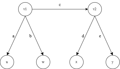
Consider all variables have the same metric (i.e., are standardized), then we have equations 1-6: \[⍴_{uw} = ab\] \[⍴_{ux} = acd\] \[⍴_{uy} = ace\] \[⍴_{xy} = de\] \[⍴_{wy} = bce\] \[⍴_{wx} = bcd\] Thus, the following equation is true: \[⍴_{ux}⍴_{wy} = ⍴_{uy}⍴_{wx}\]
and it reduces to \[(acd + abf)(bce) = (ace)(bcd + f)\] which is only an identity for particular values of \(a\), \(b\), \(c\), \(d\), \(e\), and \(f\). Thus by adding the edge \(v1 → v2\) affects the trek from \(w\) to \(x\), thus, we have defeated the implication of the tetrad equation implied by the same graph without that edge.
To give an example of a successful tetrad equation in a factor model, see the example from Figure 3.7. Imagine a tetrad equation for a unidimensional factor model with 4 items. The factor model assumes no causal relation between indicators (e.g, \(x1 → x2\) does not exist). In addition, if any trek between two measured variables contributes to the correlation between those variables, and the contribution from any trek is the product of the linear coefficients along that trek, then the correlation between any two measured variables \(x1\) and \(x2\) can be understood as the product of factor loadings \(𝜆_1\) and \(𝜆_2\), which is (i.e., \(⍴_{12} = 𝜆_1𝜆_2\)). Thus, the implied tetrads \(⍴_{12}⍴_{34}=⍴_{13}⍴_{24}=⍴_{14}⍴_{32}\) is true.
It is essential to recognize that constraints on the covariance or correlation matrix reflect the claims a model or theory makes about its domain of application. However, there is no guarantee that the measured covariance values will align with these constraints. If the model is entirely accurate, the population covariances should adhere to the restrictions it implies. Thus, when applying a reflective model such as factor analysis, the covariances should adhere to the causal relations and its’ restrictions.
When evaluating a model or comparing alternative models, the key consideration is that these constraints represent testable implications about measurable aspects of the population. Constraints on covariances can take various forms, such as: (1) Certain covariances being equal to zero. (2) Specific covariances being equal to one another. (3) Certain partial correlations being zero. (4) Particular partial correlations being equal to each other. (5) Tetrad equations. (6) Higher-order equations, such as sextet equations. Among these, tetrad equations are the most commonly encountered constraints in multiple indicator models, making them particularly significant in this context (Glymour & Scheines, 1986). (Glymour & Scheines, 1986). To see other ways to test the causal structure of your instrument, see the article by Franco et al., (2023).
3.7.1 Vanishing Tetrads in R
I’ll use as an example a reflective model (i.e., factor model) of a Openness personality measure. If the tetrads vanishes for this measure, we’ll have evidence of causality from the latent variable to the indicators, which means that the factor model might be an appropriate model.
We have an R function that does the calculations of vanishing tetrads.
You can use and install the R package that does this:
# install and load devtools to be able to install packages from GitHub with install_github
install.packages("devtools")
library(devtools)

# install CauseAndCorrelation from Bill's GitHub
install_github("BillShipley/CauseAndCorrelation")
library(CauseAndCorrelation)
?Causal.Inference
However, since there’s a problem in the R package in the day I’m writing this (due to the dependency on package graph, that is currently out of CRAN), I’ll copy the specific function we’ll use from their GitHub.
vanishing.tetrads<-function (dat, sig = 0.05)
{
    get.3.equations <- function(tet.vector) {
        mat <- matrix(NA, ncol = 8, nrow = 3)
        mat[1, ] <- cbind(tet.vector[1], tet.vector[2], tet.vector[3],
            tet.vector[4], tet.vector[1], tet.vector[4], tet.vector[2],
            tet.vector[3])
        mat[2, ] <- cbind(tet.vector[1], tet.vector[3], tet.vector[2],
            tet.vector[4], tet.vector[1], tet.vector[4], tet.vector[2],
            tet.vector[3])
        mat[3, ] <- cbind(tet.vector[1], tet.vector[3], tet.vector[2],
            tet.vector[4], tet.vector[1], tet.vector[2], tet.vector[3],
            tet.vector[4])
        mat
    }
    test.stat <- function(dat, triplet) {
        t.vars <- sort(triplet[1:4])
        r <- var(dat, na.rm = T)
        tao <- r[triplet[1], triplet[2]] * r[triplet[3], triplet[4]] -
            r[triplet[5], triplet[6]] * r[triplet[7], triplet[8]]
        D13 <- det(r[c(triplet[1], triplet[3]), c(triplet[1],
            triplet[3])])
        D24 <- det(r[c(triplet[2], triplet[4]), c(triplet[2],
            triplet[4])])
        D <- det(r[triplet[1:4], triplet[1:4]])
        N <- dim(dat)[1]
        tao.var <- (D13 * D24 * (N + 1)/(N - 1) - D) * (1/(N -
            2))
        if (tao.var <= 0) {
            cat("triplet: ", triplet, "\n")
            cat("variance of tao is ", tao.var, "\n")
            cat("tao.var<=0. D=", D, "D13=", D13, "D24=", D24,
                "\n")
            stop()
        }
        z <- tao/sqrt(tao.var)
        list(triplet = triplet, VCV = r, tao = tao, tao.var = tao.var,
            z = z, prob = 2 * (1 - pnorm(abs(z))))
    }
    get.choke.points <- function(vec) {
        tetrad <- matrix(vec, ncol = 2, byrow = T)
        all.comb <- cbind(c(vec[1], vec[1], vec[1], vec[2], vec[2],
            vec[3]), c(vec[2], vec[3], vec[4], vec[3], vec[4],
            vec[4]))
        chokes <- rep(T, 6)
        for (j in 1:4) {
            for (i in 1:6) {
                if (sum(tetrad[j, ] == all.comb[i, c(1, 2)]) ==
                  2)
                  chokes[i] <- F
                if (sum(tetrad[j, ] == all.comb[i, c(2, 1)]) ==
                  2)
                  chokes[i] <- F
            }
        }
        list(tetrad = tetrad, all.comb = all.comb, choke.points = all.comb[chokes,
            ])
    }
    nvars <- dim(dat)[2]
    tetrad.quadriplets <- combn(1:nvars, 4)
    ntetrads <- dim(tetrad.quadriplets)[2]
    z <- prob <- rep(NA, ntetrads * 3)
    count <- 0
    for (i in 1:ntetrads) {
        triplets <- get.3.equations(tetrad.quadriplets[, i])
        for (j in 1:3) {
            count <- count + 1
            temp <- test.stat(dat, triplets[j, ])
            z[count] <- temp$z
            prob[count] <- temp$prob
            if (prob[count] <= sig)
                cat("triplet:", triplets[j, ], " does not vanish (p=",
                  prob[count], ") \n\n")
            if (prob[count] > sig) {
                chokes <- get.choke.points(triplets[j, ])
                cat("triplet:", triplets[j, ], "  vanishes (p=",
                  prob[count], ") \n")
                cat("If there is a saturated dependency graph for the four variables (via EPA):",
                  triplets[j, 1], triplets[j, 2], triplets[j,
                    3], triplets[j, 4], "\n")
                cat("then there is at least one latent common cause of either (",
                  chokes$choke.points[1, 1], ",", chokes$choke.points[1,
                    2], ") and/or of (", chokes$choke.points[2,
                    1], ",", chokes$choke.points[2, 2], ")\n\n")
            }
        }
    }
}
The package states that the vanishing.tetrads() does the following:
For each unique set of four variables in the input data, this function tests if these four variables possess “vanishing” tetrads”. A tetrad is a product of two correlations that exactly equals a second product of two correlations, each involving the same four variables. Each set of four variables has three possible tetrad equations (tetrad triplets). If a tetrad vanishes, but every variable of the four is dependent on every other, conditional on every possible set of the other variables, then there must be a latent variable generating these correlations.
First, let’s load the data from the psych R package.
First install it.
       O1              O2              O3              O4
 Min.   :1.000   Min.   :1.000   Min.   :1.000   Min.   :1.000
 1st Qu.:4.000   1st Qu.:1.000   1st Qu.:4.000   1st Qu.:4.000
 Median :5.000   Median :2.000   Median :5.000   Median :5.000
 Mean   :4.816   Mean   :2.713   Mean   :4.438   Mean   :4.892
 3rd Qu.:6.000   3rd Qu.:4.000   3rd Qu.:5.000   3rd Qu.:6.000
 Max.   :6.000   Max.   :6.000   Max.   :6.000   Max.   :6.000
 NA's   :22                      NA's   :28      NA's   :14
So, let’s calculate the vanishing tetrads with a simple function. The first argument we put the data, the second argument we put the desired p-value.
triplet: 1 2 3 4 1 4 2 3   vanishes (p= 0.4600686 )
If there is a saturated dependency graph for the four variables (via EPA): 1 2 3 4
then there is at least one latent common cause of either ( 1 , 3 ) and/or of ( 2 , 4 )

triplet: 1 3 2 4 1 4 2 3  does not vanish (p= 0.03361732 )

triplet: 1 3 2 4 1 2 3 4   vanishes (p= 0.1174989 )
If there is a saturated dependency graph for the four variables (via EPA): 1 3 2 4
then there is at least one latent common cause of either ( 1 , 4 ) and/or of ( 3 , 2 )
Since one triplet did not vanish, we cannot conclude we have the vanishing tetrad implied from the factor model assumptions.
3.8 References
Asher, H. B. (1983). Causal modeling. Sage.
Bagozzi, R. P. (1980). Causal models in marketing. Wiley.
Bartholomew, D. J. (1995). Spearman and the origin and development of factor analysis. British Journal of Mathematical and Statistical Psychology, 48(2), 211-220. https://doi.org/10.1111/j.2044-8317.1995.tb01060.x
Bartholomew, D.J. (2004). Measuring intelligence: Facts and fallacies. Cambridge University Press.
Bollen, K. A. (1989). Structural equations with latent variables (Vol. 210). John Wiley & Sons.
Bollen, K. A., & Ting, K. F. (1993). Confirmatory tetrad analysis. Sociological methodology, 147-175. https://doi.org/10.2307/271009
Borsboom, D. (2006). The attack of the psychometricians. Psychometrika, 71(3), 425-440. https://doi.org/10.1007/s11336-006-1447-6
Borsboom, D., & Cramer, A. O. (2013). Network analysis: an integrative approach to the structure of psychopathology. Annual review of clinical psychology, 9, 91-121. https://doi.org/10.1146/annurev-clinpsy-050212-185608
Borsboom, D., Mellenbergh, G.J., & Van Heerden, J. (2004). The concept of validity. Psychological Review, 111, 1061–1071. https://doi.org/10.1037/0033-295X.111.4.1061
Cronbach, L.J., & Meehl, P.E. (1955). Construct validity in psychological tests. Psychological Bulletin, 52, 281–302. https://doi.org/10.1037/h0040957
DeVellis, R. F., & Thorpe, C. T. (2021). Scale development: Theory and applications. Sage publications.
Diener, E., Wirtz, D., Tov, W., Kim-Prieto, C., Choi, D. W., Oishi, S., & Biswas-Diener, R. (2010). New well-being measures: Short scales to assess flourishing and positive and negative feelings. Social indicators research, 97, 143-156. https://doi.org/10.1007/s11205-009-9493-y
Franco, V. R., Bastos, R. V., & Jiménez, M. (2023, June). Tetrad Fit Index for Factor Analysis Models. Paper presented at Virtual MathPsych/ICCM 2023. Via mathpsych.org/presentation/1297.
Glymour, C., & Scheines, R. (1986). Causal modeling with the TETRAD program. Synthese, 68, 37-63.
Glymour, C., Scheines, R., & Spirtes, P. (2014). Discovering causal structure: Artificial intelligence, philosophy of science, and statistical modeling. Academic Press.
Hambleton, R. K., Swaminathan, H. and Rogers, H. J. (1991) Fundamentals of Item Response Theory. Sage
Harackiewicz, J. M., & Priniski, S. J. (2018). Improving student outcomes in higher education: The science of targeted intervention. Annual review of psychology, 69(1), 409-435. https://doi.org/10.1146/annurev-psych-122216-011725
Harman, H. H. (1976). Modem factor analysis (3rd ed.). University of Chicago Press.
Heise, D. R. (1975). Causal analysis. Wiley.
Herrnstein, R.J., & Murray, C. (1994). The Bell curve. The Free Press.
James, L. R., Mulaik, S. A., & Brett, J. M. (1982). Causal analysis: Assumptions, models and data. Sage.
John, O. P. (2021). History, measurement, and conceptual elaboration of the Big‑Five trait taxonomy: The paradigm matures. In O. P. John & R. W. Robins (Eds.), Handbook of personality: Theory and research (pp. 35–82). The Guilford Press.
Jonas, K. G., & Markon, K. E. (2016). A descriptivist approach to trait conceptualization and inference. Psychological Review, 123(1), 90.
Kim, J. O., & Mueller, C. W. (1978). Factor analysis. Sage.
Loken & Molenaar (2008). Categories or Continua? The Correspondence Between Mixture Models and Factor Models. In G. R. Hancock & K. M. Samuelsen (Eds), Advances in Latent Variable Mixture Models. (pp. 277 - 298).
Long, J. S. (1983). Confirmatory factor analysis: A preface to LISREL. Sage.
Lord, F. M., & Novick, M. R. (1968). Statistical theories of mental test scores. Addison-Wesley.
Lynn, R., & Vanhanen, T. (2002). IQ and the wealth of nations. Praeger.
Maraun, M. D., & Gabriel, S. M. (2013). Illegitimate concept equating in the partial fusion of construct validation theory and latent variable modeling. New Ideas in Psychology, 31(1), 32–42. https://doi.org/10.1016/J.NEWIDEAPSYCH.2011.02.006
Maraun, M. D., & Peters, J. (2005). What does it mean that an issue is conceptual in nature?. Journal of personality assessment, 85(2), 128-133. https://doi.org/10.1207/s15327752jpa8502_04
McDonald, R. P. (2013). Test theory: A unified treatment. Psychology Press.
Mellenbergh, G.J. (1989). Item bias and item response theory. International Journal of Educational Research, 13, 127–143. https://doi.org/10.1016/0883-0355(89)90002-5
Meredith, W. (1993). Measurement invariance, factor analysis, and factorial invariance. Psychometrika, 58, 525–543. https://doi.org/10.1007/BF02294825
Meredith, W., & Tisak, J. (1990). Latent curve analysis. Psychometrika, 55, 107-122. https://doi.org/10.1007/BF02294746
Messick, S. (1989). Validity. In R.L. Linn (Ed.), Educational measurement (pp. 13–103). American Council on Education and National Council on Measurement in Education.
Messick, S. (1995). Validity of psychological assessment: Validation of inferences from persons’ responses and performances as scientific inquiry into score meaning. American Psychologist, 50(9), 741-749. https://doi.org/10.1037/0003-066X.50.9.741
Michell, J. (2001). Teaching and misteaching measurement in psychology. Australian Psychologist, 36(3), 211-218. https://doi.org/10.1080/00050060108259657
Michell, J. (2014). An introduction to the logic of psychological measurement. Psychology Press.
Millsap, R.E., & Everson, H.T. (1993). Methodology review: Statistical approaches for assessing bias. Applied Psychological Measurement, 17, 297–334. https://doi.org/10.1177/014662169301700401
Moneta, A., & Russo, F. (2014). Causal models and evidential pluralism in econometrics. Journal of Economic Methodology, 21(1), 54-76. https://doi.org/10.1080/1350178X.2014.886473
Muthén, B. O., & Muthén, L. K. (2000). Integrating person-centered and variablecentered analyses: Growth mixture modeling with latent trajectory classes. Alcoholism: Clinical & Experimental Research, 24(6), 882-891. https://doi.org/10.1111/j.1530-0277.2000.tb02070.x
Nunnally, J. C. (1978). Psychometric theory (2nd ed). McGraw-Hill.
Oberski, D. (2016). Mixture models: Latent profile and latent class analysis. Modern statistical methods for HCI, 275-287. https://doi.org/10.1007/978-3-319-26633-6_12
Pechorro, P., DeLisi, M., Gonçalves, R. A., Quintas, J., & Hugo Palma, V. (2021). The Brief Self-Control Scale and its refined version among incarcerated and community youths: Psychometrics and measurement invariance. Deviant Behavior, 42(3), 425-442. https://doi.org/10.1080/01639625.2019.1684942
Schmalz, X., Breuer, J., Haim, M., Hildebrandt, A., Knöpfle, P., Leung, A. Y., & Roettger, T. B. (2024, August 21). Let’s talk about language — and its role for replicability. Retrieved from <osf.io/preprints/metaarxiv/w2gb9>
Spearman, C. (1904). ‘General intelligence’ objectively determined and measured. American Journal of Psychology, 5, 201-293. https://doi.org/10.1037/11491-006
Stanovich, K. E. (2009). What intelligence tests miss: The psychology of rational thought. Yale University Press.
Tetrick, L. E., & Winslow, C. J. (2015). Workplace stress management interventions and health promotion. Annual Review of Organizational and Psychology Organizational Behavior, 2(1), 583-603. https://doi.org/10.1146/annurev-orgpsych-032414-111341
Trendler, G. (2013). Measurement in psychology: A case of ignoramus et ignorabimus? A rejoinder. Theory & Psychology, 23(5), 591-615. https://doi.org/10.1177/0959354313490451
Uher, J. (2021). Problematic research practices in psychology: Misconceptions about data collection entail serious fallacies in data analysis. Theory & Psychology, 31(3), 411–416. https://doi.org/10.1177/09593543211014963
Uher, J. (2022). Rating scales institutionalize a network of logical errors and conceptual problems in research practices: A rigorous analysis showing ways to tackle psychology’s crises. Frontiers in Psychology, 13, 1009893. https://doi.org/10.3389/fpsyg.2022.1009893
Uher, J. (2023). What’s wrong with rating scales? Psychology’s replication and confidence crisis cannot be solved without transparency in data generation. Social and Personality Psychology Compass, 17(5), e12740. https://doi.org/10.1111/spc3.12740
Van Bork, R., Wijsen, L. D., & Rhemtulla, M. (2017). Toward a causal interpretation of the common factor model. Disputatio, 9(47), 581-601. https://doi.org/10.1515/disp-2017-0019