4 Measurement Theory: Why it is Possible to Measure Psychological Phenomena
Sometimes, on days of perfect and exact light,
When things are as real as they can possibly be,
I slowly ask myself
Why I even bother to attribute Beauty to things.
Does a flower really have beauty?
Does a fruit really have beauty?
No: they have only color and form
And existence.
Beauty is the name of something that doesn’t exist
But that I give to things in exchange for the pleasure they give me.
It means nothing.
So why do I say about things: they’re beautiful?
Yes, even I, who live only off living,
Am unwittingly visited by the lies of men
Concerning things that simply exist.
Concerning things,
How hard to be just what we are and see nothing but the visible! (Fernando Pessoa)
Understanding the numerical representation of psychological constructs is essential for advancing the field of psychology. Classical measurement techniques provide a structured framework for assessing complex human behaviors and mental processes. By employing numerical representations, researchers can enhance the validity of their studies, leading to more accurate interpretations and meaningful insights into human cognition and behavior. In this chapter, I will tell you why we should care about measurement theory in psychology by telling you about: - Psychometrics objective; - History of measurement; - How to move forward and define a quantity in psychology; - The additive conjoint measurement framework; - If Rasch Modeling Entail Measurement; - Provide the tools to test measurement axioms.
4.1 The Objective of Psychometrics
Psychometrics is the branch of psychology that is concerned with quantifying and measuring mental attributes, behavior, performance, feelings, and the like. However, psychometrics does not shy away from criticism. As explained by Sijtsma (2012), on the one hand, we have Michell (2000, 2004, 2008) and Kyngdon (2008a, 2008b), who take the position that psychometrics is inadequate for measuring psychological attributes and should be replaced by the additive conjoint measurement (Luce & Tukey, 1964). Still, according to Sijtsma (2012), this perspective requires much of contemporary psychology: its serious implementation would bring psychological research to pause. However, what is the problem with stopping psychological research to improve further such research?
On the other hand, Borsboom and Mellenbergh (2004) and Borsboom and Zand Scholten (2008) argue that modern psychometrics, in particular, item response theory (IRT; Van der Linden & Hambleton, 1997), already successfully facilitated psychological measurement. This is the statistical perspective, which makes the mistake of confusing the prescriptive structure of a statistical measurement model with the theoretical structure of the attribute of interest.
4.2 Dr. Jekyll and Mr. Hyde: Measurement and Validity
When we are measuring an attribute (e.g., personality) from a class of objects (e.g., personality instruments), we associate numbers or other mathematical entities (e.g., Likert scales) within the objects so that the properties of the attribute are faithfully represented as numerical properties (Krantz et al., 1971). This is one of the many objectives of seeking the validity of psychological instruments (e.g., AERA, APA & NCME, 2014; Borsboom, 2005).
As exposed by Bringmann and Eronen (2015), most books, manuals, or monographs on measurement and measurement theory in psychology (for example, AERA, APA & NCME, 2014; Borsboom, 2005; Kline, 2000; McDonald, 1999), the physical measurement rarely appears. In the 2014 edition of Standards for Educational and Psychological Testing, validity is the first topic discussed, and is characterized as “the most fundamental consideration in test development and test evaluation” (AERA et al., 2014, p.11 ). According to the classical definition, validity refers to the extent to which the test or instrument measures what it is intended to measure (Kline, 2000, p. 17; McDonald, 1999, p. 197), but in the contemporary validity literature, there’s no consensus on how validity should be defined (see Newton & Shaw, 2013). Some of the most prominent approaches to validity are Messick’s (1989) unified treatment of validity, where the focus is on the appropriateness of the inferences that psychologists make based on test results. The approach is based on Kane’s arguments (2001, 2006, 2013), in which validation consists in providing evidence-based arguments for interpretations of test results.
However, all concepts of validity have relationships between the construct and its score, so they depend heavily on the quantification of psychological phenomena, which tries to be covered in psychometric research. I argue that the lack of empirical foundations for psychological measurement is “Mr. Hyde” of psychometrics, a monster for some researchers who, at the same time, is “Dr. Jekyll”, one of the many sources of validity of psychological instruments. This view aligns with that of Michell (2000), who states that “if science is a cognitive enterprise, then I argue that this way of doing it is not normal. It’s pathological”.
4.2.1 History of Psychological Measurement
The pathology of psychometrics began long before this area of knowledge existed. This all started with Pythagoras, who stated that “All things are made of numbers”. This is a very strong assumption, to say that the fundamental structure of all processes in nature is quantitative. In Timaeus, Plato continues saying the same thing, saying that all things are composed of the four basic elements (earth, fire, air, and water), which, in turn, are formed by polyhedra. He continues this logic, stating that polyhedra are made of triangles, which are reducible to lines and angles, and numbers.
But we have someone to disagree with this whole thing about reducing everything to quantities. Aristotle recognized that there are quantities (numbers, sizes, areas, etc.), but there are also qualities. These qualities are not quantitative, and concern things like colors and aromas. This distinction he said was something observable, where quantitative properties had an additive structure. Qualities did not have such a structure. Thus, he developed qualitative physics.
Of course, this fight continued between those who said that everything is quantitative and those who said that not everything is. Sometime later, Galileo himself joined the team of Pythagoras and Plato:
[The universe] cannot be read until we have learnt the language and become familiar with the characters in which it is written. It is written in mathematical language, and the letters are triangles, circles, and other geometrical figures, without which means it is humanly impossible to comprehend a single word. (Galileu - II Saggiatore)
You can see the imprint of this speech to this day. People keep claiming that everything can be expressed in mathematical terms. Of course, if you number everything you associate it with mathematics. But what lies behind this thought is saying that everything in life is quantitatively measurable.
Great contemporaries from the same area as Galileo shared his views, such as Kepler and Descartes. However, this was not what made the quantitative area “win”, and rather the fact that Galileo’s physics dominated European science, taking the focus away from its rival, Aristotle’s physics.
With all this success, Galileo gave birth to the quantitative imperative. With the advent of Newton’s works, which strengthened Galileo’s quantitative views, we increasingly have more philosophers who defend this way of thinking. Kant wrote that
… In any special doctrine of nature there can be only as much proper science as there is mathematics therein (Kant, 1786, p. 7).
You can see here the birthplace of the thought that all science must be quantitative. It was just in the 19th century that Lord Kelvin (an important physicist), expressed these thoughts more concretely
When you can measure what you are speaking about, and express it in numbers, you know something about it; but when you cannot measure it, when you cannot express it in numbers, your knowledge is of a meagre and unsatisfactory kind: it may be the beginning of knowledge, but you have scarcely, in your thoughts, advanced to the stage of science, whatever the matter may be. (W. Thomson, 1891, p. 81)
Thus, this speech became the new favorite of the quantitative movement. See, Pearson (one of the darlings of psychology) used this line in 1978. And like many other areas that wanted to claim to be scientific because of quantitative thinking, psychology was no different. Back when psychology emerged in 1860, G. Fechner was also influenced by the thinking of the time about the nature of science. Fechner was a physicist who later became interested in psychological issues, such as the intensity of sensations. Although he was not the first person to attempt to measure psychological variables (perhaps it was Nicole Oresme in the 14th century), he proposed measurement methods.
Well, quantitative thinking continued in the progenitors of psychology (in this branch of psychology, in this case). Eugenicist Francis Galton, who influenced and did many studies on psychology, wrote that
…until the phenomena of any branch of knowledge have been subjected to measurement and number, it cannot assume the status and dignity of a science (1879, p.147)
His assistant and one of the first psychology professors, James McKeen Cattell, followed this line of thought:
Psychology cannot attain the certainty and exactness of the physical sciences, unless it rests on a foundation of experiment and measurement (1890, p. 373).
Even the creator of Factor Analysis, Charles Spearman, wrote that:
… great as may be the potency of this [the experimental method], or of the preceding methods, there is yet another one so vital that, if lacking it, any study is thought by many authorities not to be scientific in the full sense of the word. This further and crucial method is that of measurement. (1937, p. 89).
E. B. Titchener (1905, pp. xxi-xxii) and Kulpe (1895, p. 11) thought the same, but stating that mental processes were measurable. Few who claimed that psychology was a science actually questioned the idea that it could be quantitative. This was probably because the status of science could be lost. A psychologist dared to do this: Franz Brentano. He adhered a little to the Aristotelian thoughts.
Mathematics appears to me necessary for the exact treatment of all sciences only because we now in fact find magnitudes in every scientific field. If there were a field in which we encountered nothing of the sort, exact description would be possible even without mathematics. (Brentano, 1874, p. 65)
S. S. Stevens, “solved” the tension between people who considered and those who did not consider psychology as a science. Stevens saw that not only additivity could be represented numerically, and placed a new emphasis on these representations. It was Stevens who popularized the concepts of nominal, ordinal, interval, and ratio scales. In 1946 (p. 667), 1951 (p. 1), and 1959 (p. 19), Stevens defined measurement as “..the assignment of numbers to objects or events according to rules”. This is one of the most famous measurement definitions in psychology today. You can find it as the main definition in thousands of psychology and psychometrics books.
However, his definition is empty of meaning. Not only are all things measurable, but also all things that can be numbered are forms of measurement. Furthermore, the distinction between quantitative and qualitative variables vanished. In other words, the variable being quantitative is no longer a characteristic of the variable itself, rather it is a pragmatic issue, decided by the researcher. Steven’s definition confuses two distinct practices: a) measurement (in the classical sense); and b) numerical coding. Measurement involves the discovery of empirical facts of an intrinsic numeric type. b) Numerical coding is simply a cosmetic use in analysis and presentation of something that is not numeric. It is just a symbolic representation of facts.
4.3 How to Move Forward: Defining Quantity
After all this confusion, we still haven’t defined what is a quantity. What distinguishes a quantitative variable from a non-quantitative one? To be quantitative, the variable must be ordered and have an additive structure. Let’s do it in steps.
What would be a variable? In general, it is anything relative to which objects can vary. Size is a variable, as different objects have different sizes. Color is a variable, given that we have several colors. Being more detailed about this, the class of variables (size, color, etc.) can only be presented once for each object. Therefore, I do not have two heights at the same time. This is a condition crucial for a variable: not owning the same property more than once. Of course, we can have different properties on the same object, such as being a tall, white, brown-haired person. We have 3 variables (height, race/ethnicity, and hair color). But that’s not all that characterizes a variable.
Relationships also form variables. The difference between properties and relationships is important. Things have uniquely shaped properties, like the size of my pen is one. Relationships involve a plurality of things. If the pen is on a table, then the situation involves both the pen and the table. Another example is speed. The speed of \(X\) relative to \(Y\) is something that involves \(X\) and \(Y\). Of course, the speed of \(X\) relative to \(Y\) is just one. But we can also have another speed, that of \(X\) in relation to \(Z\). This does not mean that \(X\) has more than one speed at the same time, it only has one, but there is also a relationship between the objects \(X\), \(Y\), and \(Z\).
Another important concept is that of value: the properties and relationships that constitute a variable can be called values of that variable. For example, being 6 meters in size is the value of the size variable. Being a woman is the value of the gender variable, and so on. When we say that a quantitative variable is ordered and additive, we are saying that there are ordinal and additive relationships between the values of that variable.
What constitutes an ordered variable? Well, a simple way is to think that 6 meters is greater than 2 meters. We can also think about education, where higher education is more education than secondary education, which in turn is more than elementary education. More concretely, the values of the variables are ordered according to their magnitudes. We use the symbol \(≥\), which means “greater than or at least equal to”, and \(>\) meaning “greater than”. The symbol \(=\) means “equal to” or “identity of the value”. Now let’s go to the mathematics of the thing.
Consider that \(X\), \(Y\) and \(Z\) are three values of a variable \(Q\). Then, \(Q\) is ordinal if and only if:
if \(𝑋 ≥ 𝑌\) and \(𝑌 ≥ 𝑍\), then \(𝑋 ≥ 𝑍\) (this property is called transitivity. It means that if \(𝑋\) is greater than or equal to \(Y\), and \(𝑌\) is greater than or equal to \(𝑍\), then \(𝑋\) must be greater than or equal to \(Z\), given the first relations mentioned).
if \(𝑋 ≥ 𝑌\) and \(𝑌 ≥ 𝑋\), then \(𝑋 = 𝑌\) (also called antisymmetry. It means that If \(𝑋\) is greater than \(𝑌\), and \(𝑌\) is greater than \(𝑋\), how can they not be greater than the other at the same time, so they have to be the same).
either \(𝑋 ≥ 𝑌\) or \(𝑌 ≥ 𝑋\) (called strong connectedness; only one variable can be larger, or both are the same).
The relation that has these 3 properties is called the simple order. \(Q\) is a ordinal variable if and only if \(≥\) is a simple order of its values. All quantitative variables are ordered by \(≥\), but not every ordinal variable is quantitative. To do this, it is necessary to have additivity.
Additivity is a ternary relationship (made up of 3 parts), symbolized as \(𝑋 + 𝑌 = 𝑍\).
Consider that \(Q\) is an ordinal variable, which for any values \(𝑋\), \(Y\), and \(𝑍\) we have:
\(X + (𝑌 + 𝑍) = (𝑋 + 𝑌 ) + 𝑍\) (associativity; i.e., the order of the sum does not affect the value resulting from the sum)
\(𝑋 +𝑌 = 𝑌 +𝑋\) (commutativity; i.e., the order of the operands does not affect the final result).
\(𝑋 ≥ 𝑌\) if and only if \(𝑋 + 𝑍 ≥ 𝑌 + 𝑍\) (monotonicity; that is, if we add the same value on both sides, in \(𝑋\) and \(𝑌\), their order continues in the same direction, where \(𝑋\) is greater than or equal to \(𝑌\)).
If \(𝑋 ≥ 𝑌\) then there is a value \(𝑍\) that makes \(𝑋 = 𝑌 + 𝑍\) (solvability; means that if a value \(𝑋\) is greater than the value \(𝑌\), there is a third value \(𝑍\) which added to \(𝑌\) makes it a value equal to \(𝑋\)).
\(𝑋 + 𝑌 ≥ 𝑋\) (positivity; if \(X\) is increased by a value \(𝑌\), then this result has be greater than the original value of \(𝑋\), given that they are ordinal variables).
there is a natural number \(n\) such as \(n𝑋 ≥ 𝑌\) (where \(1𝑋 = 𝑋\) and \((𝑛+1)𝑋 = 𝑛𝑋+𝑋\) (Archimedean Condition; means that no value \(𝑌\) of the variable is infinitely greater than any other variable \(𝑋\)).
These nine conditions (ordinal and additive) are uniformly coexisting. What it means is that they do nothing other than describe the structure of the variable. It does not describe the behavior of objects that have values of this variable.
Thus, it is not just additivity that a measure lives on. But an important criticism of Michell is how psychometricians do not evaluate their models correctly, at the level of measurement theory. As a result, they assume many things that may or may not be true, requiring testing or theorizing about these created measures. If psychometricians really evaluated the level of measurement of their variables, this would already solve the problem of psychometrics being pathological. We cannot keep assuming things that can be testable, or at least theorized in a more concrete way.
4.3.1 Additive Conjoint Measurement
The defense of the Additive Conjoint Measurement will be expressed here according to Michel (2014). Luce and Tukey (1964) proposed the additive conjoint measurement (ACM) specifically for quantification within the social sciences. This measure theory provides a way to identify quantitative structure other than through concatenation (or physical addition) operations. Instead, it allows quantitative structure to be detected through ordinal relationships on a variable. Although psychology lacks concatenation operations, it has many ordinal relationships.
The theory is about the type of situation in which a quantitative variable, 𝑃, is a non-interactive function of two other variables, \(A\) and \(𝑋\). The word “non-interactive” can be understood as “additive” or “multiplicative”, although, in fact, it is more general than that. This means that conjoint measurement theory refers to situations like \(𝑃 = 𝐴 + 𝑋\), or \(𝑃 = 𝐴 ∗ 𝑋\). Its application is specifically to those instances where no \(P\), \(𝐴\), or \(𝑋\) are already quantified. This requires that:
the variable \(𝑃\) has an infinite number of values;
\(𝑃 = 𝑓(𝐴, 𝑋)\) (where \(𝑓\) is some mathematical function);
there is a simple order over the values of \(P\); and
the values of \(𝐴\) and \(X\) can be identified (i.e. objects can be classified according to the value of \(𝐴\) and \(𝑋\)).
Let us call a system that satisfies (i)-(iv) a conjoint system. So if \(≥\) in \(𝑃\) satisfies three special conditions, it follows that:
- \(𝑃\), \(𝐴\), and \(𝑋\) are quantitative; and
- \(𝑓\) is a non-interactive function.
The three special conditions are:
Double Cancellation;
Solvability; and
the Archimedean condition;
Suppose \(P\) is performance on some task (say, the time it takes to run a maze), \(𝐴\) is motivation, and \(𝑋\) is the amount of prior practice. Of course, it would be a simple matter to order the performances and classify subjects according to motivation (e.g., duration of food or water deprivation) and number of previous practice attempts.
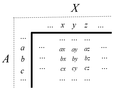
Such conjoint systems are easily visually contemplated if they are thought of as composing a matrix where the rows are values of \(A\), the columns, values of 𝑋, and the cells, values of \(𝑃\). Let \(𝑎\), \(𝑏\), \(𝑐\),… etc. be values of \(𝐴\), \(𝑥\), \(𝑦\), \(𝑧\),… etc. be values of \(𝑋\) and, since \(𝑃 = 𝑓(𝐴, 𝑋)\), the pairs, \(𝑎𝑥\), \(𝑎𝑦\),… , \(𝑐𝑦\), \(c𝑧\),… denote (possibly identical) values of \(P\). Such a matrix is schematically represented by Figure 4.1 to help understand a visual representation of conditions (1) - (3).
4.3.1.1 Double Cancelation
The double cancellation condition states that if certain pairs of values of \(𝑃\) are ordered by \(≥\), other pairs of specific values will also be ordered. It’s like the transitivity condition that ≥ must satisfy (being a simple order). In the context of conjoint measurement, the transitivity of \(≥\) in \(P\) is a special case of double cancellation.
Double cancellation takes the following form. Let \(𝑎\), \(𝑏\), and \(𝑐\) be any values of \(𝐴\) and \(x\), \(𝑦\), and \(𝑧\) be any values of \(𝑋\), then \(≥\) in \(𝑃\) satisfies double cancellation if and only if
\[ \text{we have}\ ay ≥ bx \\ \] \[ \text{and also have}\ bz ≥ cy \\ \] \[ \text{thus,}\ az ≥ cx. \] Thus the condition appears obscure, but some light is shed if double cancellation is seen as a consequence of that special case of a non-interactive relation between \(𝑃\), \(𝐴\), and \(𝑋\),
\[ P = A + X. \]
Given this relation,
\[ ay ≥ bx\ \text{if and only if}\ a + y ≥ b + x \] \[ \text{and}\ bz ≥ ey\ \text{if and only if}\ b + z ≥ e + y. \] Adding the two inequalities on the right-hand side we get
\[ a+y+b+z ≥ b+x+c+y \]
and since \(𝑏\) and \(𝑦\) is common on both sides of the inequality, they can be canceled, leaving
\[a + z ≥ c + x\]
which, of course, is true if and only if
\[az ≥ cx\].
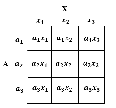
Despite its simplicity, double cancellation is a condition that has considerable power. It strongly restricts the order in \(P\). This can be illustrated in a \(3𝑋3\) matrix. Let \(𝑎1\), \(𝑎2\), and \(𝑎3\) be three values of \(𝐴\) and \(𝑥1\), \(𝑥2\) and \(𝑥3\) be three values of \(𝑋\). The resulting conjoint matrix is illustrated in Figure 4.2.
Now, because \(a\), \(b\), and \(c\) in the double cancellation condition are any values of \(A\), then \(a1\), \(a2\) and \(a3\) can be substituted for them in any of the 3! (= 6) different possible ways. Similarly, \(x1\), \(x2\) and \(x3\) can be replaced by \(x\), \(y\) and \(z\) in 6 different ways. This produces 6 x 6 (= 36) different substitution instances of the double cancellation condition in the 3 x 3 matrix shown above (or in any 3 x 3 conjoint matrix). These 36 different replacement instances are shown in Figure 4.3.
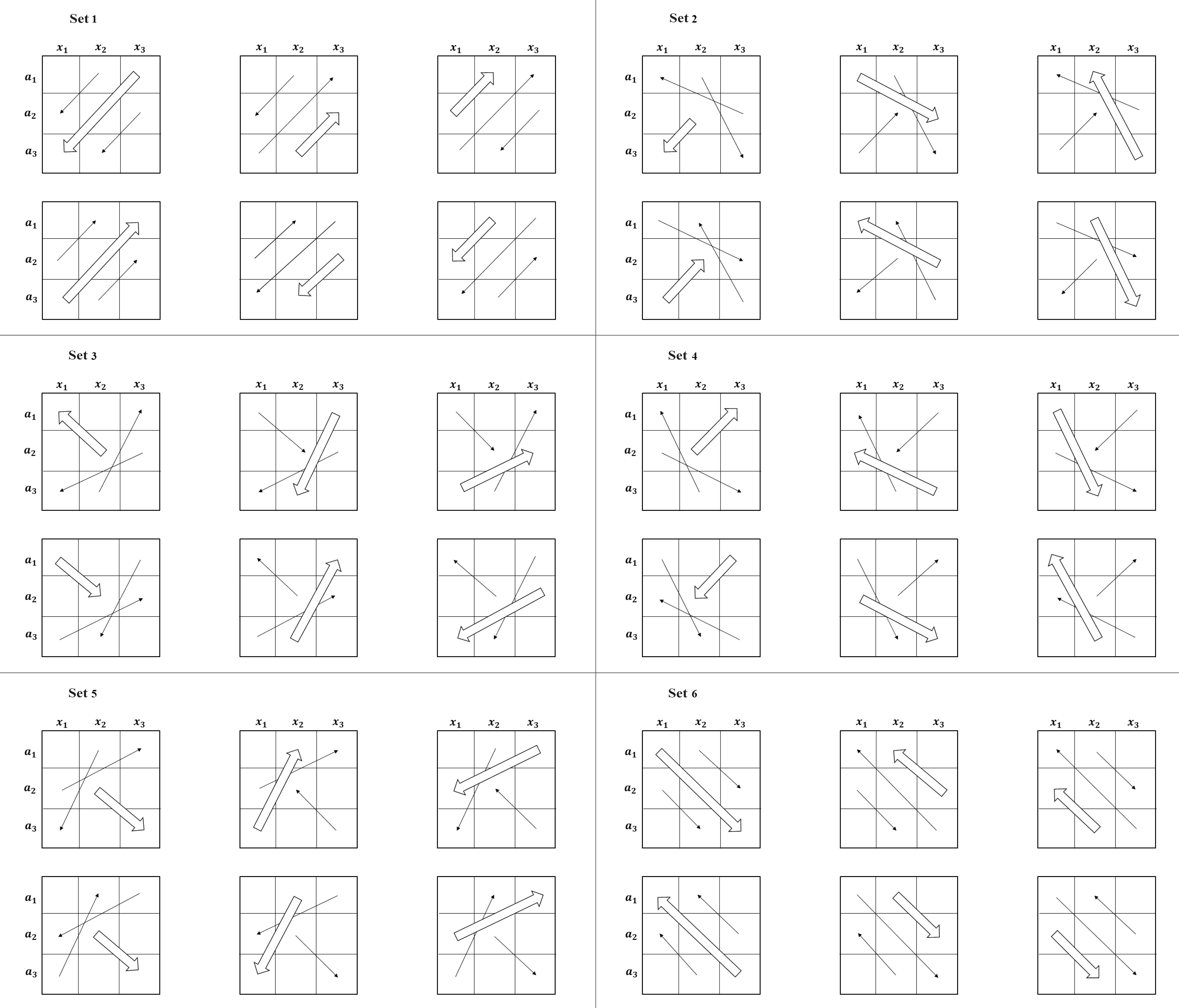
They are not all logically independent of each other. In this, they are in six different sets, each with six. Within each set, the relevant order relations are between the same three values of \(𝑃\) (or matrix cells). Arrows have been used to indicate these relationships (i.e., \(𝑎𝑥 ≥ 𝑏𝑦\) is represented by \(ax\) -> \(by\) , the single-line arrows represent the antecedent orders and double-line arrows represent the consequent order.
Within each set of six, if one of the double cancellation instances is true, they all will be. However, between sets, instances of double cancellation are logically independent of each other. Thus, within any 3 x 3 matrix there are six independent tests of the double cancellation condition, this condition is false if in any of the diagrams shown in the figure above, the antecedent order relations are valid, while the consequent is not; otherwise, they are satisfied. Obviously, satisfying double cancellation (in a conjoint matrix, even a 3 x 3 one) is not a trivial issue and very computationally demanding.
4.3.1.2 Solvability
The solvability condition requires that the variables \(𝐴\) and \(𝑋\) are complex enough to produce any required value of \(𝑃\). It is formally stated as the following.
The order \(≥\) in 𝑃 satisfies solvability if and only if (i) for any \(𝑎\) and \(b\) in \(𝐴\) and \(x\) in \(𝑋\), there is a value of \(𝑋\) (call it \(𝑦\)) such that \(𝑎𝑥 = 𝑏𝑦\) (i.e., both \(a𝑥 ≥ 𝑏𝑦\) and \(𝑏𝑦 ≥ 𝑎𝑥\)); and (ii) for any \(𝑥\) and \(𝑦\) in \(𝑋\) and \(𝑎\) in \(𝐴\), there is a value of \(𝐴\) (call it \(𝑏\)) such that \(𝑎𝑥 = 𝑏𝑦\). In other words, given any \(𝑎\), \(𝑏\), \(𝑥\), and \(𝑦\), \(𝑦\) exists such that the equation
\[ ax = by \] is solvable.
Thinking in terms of the relationship \(𝑃 = 𝐴 + 𝑋\), solvability implies that the values of \(𝐴\) and \(X\) they are equally spaced (as natural numbers are) or they are dense (as rational numbers are).
4.3.1.3 Achimedean Condition
As already explained, the Archimedean condition guarantees that no value of a variable quantity is infinitely greater than any other value. Its meaning here is essentially the same, although in this context its expression is a little more complex. Thinking again in terms of \(𝑃 = 𝐴 + 𝑋\), a general idea of its content can be stated as follows. Conjoint measurement allows the quantification of differences between the values of \(A\), between the values of \(𝑋\), and between the values of \(P\). Limiting attention to \(𝐴\), the Archimedean condition means that no difference between any two values of \(𝐴\) is infinitely greater than the difference between any other two values of \(𝐴\).
4.4 The Tale of Taxometric Analysis
The taxometric method started by Meehl (1995) is designed to assist researchers in determining whether the latent structure of a variable is categorical or continuous (Ruscio et al., 2007). The logic behind such analysis, regardless of the different way of performing it, relies on identifying if the latent distribution is unimodal or multimodal. If the former its’ discovered, the researcher will conclude that the measurement level is continuous. In contrast, if the latter is found to be true, there will be evidence in favor of a categorical measurement level (Franco, 2021).
Ruscio and Kaczetow (2009) showed through extensive simulation studies that the curve-comparison fit indexes can identify the measurement level of a latent trait with 93% accuracy. However, in publications using such method, a meta-analysis showed a tendency of studies showing evidence in favor of a numerical and against a categorical latent variable (Haslam et al., 2012). Some possible limitations of taxometrics are due to its’ lack of robustness both in statistical and measurement theory. For instance, its’ hard to interpret taxometric analysis because the structure of observed covariance allows identical model fit with K taxons in comparison of models with K – 1 factors (Gibson, 1959), which makes taxometric analysis an unfalsifiable method. Moreover, this method has no further developments on current measurement theory, such as testing assumptions of ACM under the psychometric theory.
4.5 Does Rasch Modeling Entail Measurement?
In order to derive a numerical representation of psychological variables, a series of analyses have been developed. Still, conjoint measurement had very little impact on the construction of these psychometric models (Cliff, 1992; Narens & Luce, 1993; Ramsay, 1975, 1991; Schwager, 1991). One of these models is constantly related to conjoint measurement, the Rasch (1960) modeling.
To relate the Rasch model with conjoint measurement, some authors mistakenly argue the relationship via analogy with physical measurement (Kyngdon, 2008a). For instance, Fischer (1995) reached the conclusion that due to the logarithmic transformations yielding additive connections between derived measurements in physics, it logically follows that the constructs of individual ability and item complexity possess adequate complexity to support representation theorems extending to real numbers, which are essentially unique barring linear adjustments. In essence, individual ability and item difficulty are deemed to exhibit additive structures solely based on altering the relationship between these constructs. This relationship, however, is held by analogy to derived measurement through the notion of specific objectivity (Kyngdon, 2008a). To assert that an additive interval measurement of a person’s ability and item difficulty is given by Rasch (1960), it’s required that the underlying assumption is true: test performance is a multiplicative conjoint structure comprising of a person’s ability and the item difficulty. Nonetheless, this has not been proven elsewhere.
Most research regarding the connection between Rasch modeling and conjoint measurement states that the Rasch model is a probabilistic version of conjoint measurement (Kyngdon, 2008b; e.g., Borsboom & Mellenbergh, 2004; Karabatsos, 2001; Kline, 1998). Thus, data that fits the Rasch model should allow for interval scaling. However, this is controversial. As stated by Michel (2008), the theory of conjoint measurement is a theory of ordinal and equivalence relations necessary for quantification, while the Rasch model is not concerned with such relations. Thus, the lack of articulation between Rasch and these relations does not entail that Rasch is mathematically equivalent to the theory of conjoint measurement (Kyngdon, 2008b). The difference between Rasch and the theory of conjoint measurement is mathematically clear. The theory of conjoint measurement proposes axioms for order and additivity (Luce & Tukey, 1964), while Rasch only proposes ordering of persons and items (Borsboom & Zand Scholten, 2008).
In standard research practice, when a person runs a Rasch model, they supposedly check for the consistency between the data and model with measurement axioms using fit statistics (Karabatsos, 2001). However, even if we assume that Rasch is testing those axioms, the test using fit statistics is not straightforward, since the specification of additive conjoint measurement under the Rasch model is data-dependent. This is because the Item Response Function is estimated directly from data, and data contains random or systematic noise. A consequence of such an effect is shown by Nickerson and McClelland (1984) and Karabastos (2001), where they show that Rasch modeling can empirically show perfect data fit, even for data sets containing violations of conjoint measurement axioms.
4.5.1 Representationally Adequate Item Response Theory Models
Scheiblechner (1995, 1998) developed the Isotonic Ordinal Probabilistic Model (ISOP) to address limitations in the Rasch model. ISOP operates on the premise that in Experimental or Testing Psychology, it is common to hypothesize an ordinal variable before experiments, allowing the ranking of observed reactions. This model fits by testing axioms I and II from additive conjoint measurement theory and is often referred to as a probabilistic version of Guttman scaling or an implementation of Mokken scaling, as suggested by Molenaar (1991).
Unlike parametric latent trait models, ISOP is nonparametric, meaning it doesn’t rely on a specific parametric family, functional curve form, or prior distribution of latent ability. It is based on axiomatic principles, with independent and separately testable axioms, offering nonparametric statistical tests for various unidimensional models. This structure enables ISOP to distinguish between poor fit caused by latent trait multidimensionality and poor parameterization.
The ISOP model provides a foundational framework in measurement theory, emphasizing ordinal unidimensionality and offering algorithms and technologies for test development. It assumes that responses are generated by the interaction of individuals and items, producing a common ordinal scale, but the effects are not additive. Scheiblechner (1999) extended ISOP by incorporating the cancellation axiom (axiom III), resulting in the Additive Conjoint Isotonic Probabilistic Model (ADISOP). This extension allows for the creation of two ordered metric scales with a shared unit for both subjects and items, enabling an additive representation of latent variables that interact to produce the observed orders.
Although ADISOP shares similarities with the Rasch model, it does not prescribe a specific item response function. Scheiblechner (1999) suggests that comparing ISOP, ADISOP, and the Rasch model can help assess the measurement level of latent variables. These models form a hierarchy, transitioning from ordinal to interval measures (if ADISOP fits better than ISOP) and from interval measures with uncertainty to those with a strong functional form (if the Rasch model fits better than ADISOP).
4.6 The Direct Test of Conjoint Measurement Axioms
A Bayesian technique originated in Karabatsos (2001) and further developed by Domingue (2013) makes it possible to test the ACM axioms. Suppose there’s a unidimensional latent variable, which has a function linking the persons’ responses to a set of items. Consider that \(P\) is an \(I x J\) matrix that contains the true response probabilities for this set of items. Each cell in the conjoint matrix \(P^{MLE}\), with dimensions \(I x J\), contains the percentage of respondents with a certain ability who answered the appropriate item correctly.
In order to determine whether the axioms are true for \(P\), the order restrictions from the cancellation axioms are imposed stochastically via the Metropolis-Hastings (Metropolis et al., 1953; Hastings, 1970) jumping distribution. Domingue (2013) conducted simulation studies to test the new approach, and the evidence suggests that this approach can discriminate between data generated via the Rasch model and the 3PL model. This is expected, given that the 3PL item response model does not follow the axioms of additive conjoint measurement.
There is an R package called ConjointChecks (Domingue, 2013) that tests the assumptions regarding the cancellation of the additive conjoint measures. To download it, you need the updated devtools library, and install the most current version of the package.
4.7 ISOP and ADISOP Model
To fit an ISOP or ADISOP model, we must first install the sirt package, and the psych package for the dataset.
So, we tell the program that we are going to use the functions of these packages.
To run the analyses, we will use a unidimensional subset of the BFI database (Big Five Personality Factors Questionnaire) that already exists in the psych package. We also need to reverse code the first item, because it’s inverted.
4.7.1 Fitting ISOP and ADISOP models
The function to fit ISOP and ADISOP models is quite simple. We just need the put the data variable (with only the important items) inside one of sirt functions. Since we are dealing with an polytomous scale, we will use the isop.poly function. If you are dealing with dichotomous scales, use the isop.dich function.
Fit ISOP Category 0
*******ISOP Model***********
Iteration 1 - Deviation= 0

Fit ISOP Category 1
*******ISOP Model***********
Iteration 1 - Deviation= 5.811229
Iteration 2 - Deviation= 0.000549
Iteration 3 - Deviation= 3e-06

Fit ISOP Category 2
*******ISOP Model***********
Iteration 1 - Deviation= 11.83981
Iteration 2 - Deviation= 0

Fit ISOP Category 3
*******ISOP Model***********
Iteration 1 - Deviation= 12.84252
Iteration 2 - Deviation= 0

Fit ISOP Category 4
*******ISOP Model***********
Iteration 1 - Deviation= 12.62383
Iteration 2 - Deviation= 0

Fit ISOP Category 5
*******ISOP Model***********
Iteration 1 - Deviation= 24.90762
Iteration 2 - Deviation= 0

*******ADISOP Model*********
Iteration 1 - Deviation= 1.910899
Iteration 2 - Deviation= 0.18115
Iteration 3 - Deviation= 0.129763
Iteration 4 - Deviation= 0.095663
Iteration 5 - Deviation= 0.072329
Iteration 6 - Deviation= 0.055969
Iteration 7 - Deviation= 0.045332
Iteration 8 - Deviation= 0.040025
Iteration 9 - Deviation= 0.03533
Iteration 10 - Deviation= 0.031179
Iteration 11 - Deviation= 0.027513
Iteration 12 - Deviation= 0.024281
Iteration 13 - Deviation= 0.021436
Iteration 14 - Deviation= 0.018932
Iteration 15 - Deviation= 0.016795
Iteration 16 - Deviation= 0.014916
Iteration 17 - Deviation= 0.013255
Iteration 18 - Deviation= 0.011783
Iteration 19 - Deviation= 0.010476
Iteration 20 - Deviation= 0.009314
Iteration 21 - Deviation= 0.008282
Iteration 22 - Deviation= 0.007364
Iteration 23 - Deviation= 0.006548
Iteration 24 - Deviation= 0.005823
Iteration 25 - Deviation= 0.005177
Iteration 26 - Deviation= 0.004604
Iteration 27 - Deviation= 0.004094
Iteration 28 - Deviation= 0.00364
Iteration 29 - Deviation= 0.003237
Iteration 30 - Deviation= 0.002878
Iteration 31 - Deviation= 0.002559
Iteration 32 - Deviation= 0.002275
Iteration 33 - Deviation= 0.002023
Iteration 34 - Deviation= 0.001799
Iteration 35 - Deviation= 0.0016
Iteration 36 - Deviation= 0.001422
Iteration 37 - Deviation= 0.001265
Iteration 38 - Deviation= 0.001124
Iteration 39 - Deviation= 0.001
Iteration 40 - Deviation= 0.000889
Iteration 41 - Deviation= 0.00079
Iteration 42 - Deviation= 0.000703
Iteration 43 - Deviation= 0.000625
Iteration 44 - Deviation= 0.000556
Iteration 45 - Deviation= 0.000494
Iteration 46 - Deviation= 0.000439
Iteration 47 - Deviation= 0.000391
Iteration 48 - Deviation= 0.000347
Iteration 49 - Deviation= 0.000309
Iteration 50 - Deviation= 0.000274
Iteration 51 - Deviation= 0.000244
Iteration 52 - Deviation= 0.000217
Iteration 53 - Deviation= 0.000193
Iteration 54 - Deviation= 0.000172
Iteration 55 - Deviation= 0.000153
Iteration 56 - Deviation= 0.000136
Iteration 57 - Deviation= 0.000121
Iteration 58 - Deviation= 0.000107
Iteration 59 - Deviation= 9.5e-05

*******Graded Response Model***********
Iteration 0 - Deviation= 1
Iteration 1 - Deviation= 0.990099
Iteration 2 - Deviation= 0.694234
Iteration 3 - Deviation= 0.611731
Iteration 4 - Deviation= 0.682299
Iteration 5 - Deviation= 0.67898
Iteration 6 - Deviation= 0.64934
Iteration 7 - Deviation= 0.614304
Iteration 8 - Deviation= 0.572969
Iteration 9 - Deviation= 0.527128
Iteration 10 - Deviation= 0.478988
Iteration 11 - Deviation= 0.430309
Iteration 12 - Deviation= 0.382417
Iteration 13 - Deviation= 0.336313
Iteration 14 - Deviation= 0.292744
Iteration 15 - Deviation= 0.252246
Iteration 16 - Deviation= 0.215173
Iteration 17 - Deviation= 0.181717
Iteration 18 - Deviation= 0.151937
Iteration 19 - Deviation= 0.125775
Iteration 20 - Deviation= 0.103086
Iteration 21 - Deviation= 0.083652
Iteration 22 - Deviation= 0.067209
Iteration 23 - Deviation= 0.053463
Iteration 24 - Deviation= 0.042107
Iteration 25 - Deviation= 0.032835
Iteration 26 - Deviation= 0.025352
Iteration 27 - Deviation= 0.01938
Iteration 28 - Deviation= 0.014668
Iteration 29 - Deviation= 0.010992
Iteration 30 - Deviation= 0.008156
Iteration 31 - Deviation= 0.005992
Iteration 32 - Deviation= 0.004359
Iteration 33 - Deviation= 0.00314
Iteration 34 - Deviation= 0.002239
Iteration 35 - Deviation= 0.001582
Iteration 36 - Deviation= 0.001106
Iteration 37 - Deviation= 0.000766
Iteration 38 - Deviation= 0.000526
Iteration 39 - Deviation= 0.000358
Iteration 40 - Deviation= 0.000241
Iteration 41 - Deviation= 0.000161
Iteration 42 - Deviation= 0.000107
Iteration 43 - Deviation= 7.1e-05 -----------------------------------------------------------------
sirt 4.1-15 (2024-02-06 00:05:40)
Date of Analysis: 2025-01-30 14:27:23.960409
ISOP and ADISOP Model
-----------------------------------------------------------------
Number of persons= 2709
Number of items= 5
Number of person score groups= 9
Number of item score groups= 5
Log-Likelihood Comparison
model ll llcase
1 saturated -15894.56 -5.86732
2 isop -16171.19 -5.96943
3 adisop -16300.51 -6.01717
4 grm -16571.02 -6.11702
*****************************************************************
Item Statistics and Scoring
item M pscore p.Cat0 p.Cat1 p.Cat2 p.Cat3 p.Cat4 p.Cat5 p.Cat6
A1- A1- 4.5877 0.0105 0 0.0292 0.0797 0.1211 0.1440 0.2964 0.3296
A2 A2 4.7973 0.0775 0 0.0173 0.0461 0.0546 0.1993 0.3688 0.3138
A3 A3 4.5991 -0.0577 0 0.0329 0.0624 0.0753 0.2027 0.3559 0.2709
A4 A4 4.6822 0.0612 0 0.0476 0.0790 0.0664 0.1643 0.2359 0.4068
A5 A5 4.5511 -0.0915 0 0.0218 0.0676 0.0919 0.2219 0.3503 0.2466
score.Cat0 score.Cat1 score.Cat2 score.Cat3 score.Cat4 score.Cat5
A1- -1 -0.9708 -0.8619 -0.6611 -0.3961 0.0443
A2 -1 -0.9827 -0.9192 -0.8184 -0.5644 0.0037
A3 -1 -0.9671 -0.8719 -0.7342 -0.4563 0.1023
A4 -1 -0.9524 -0.8258 -0.6803 -0.4496 -0.0495
A5 -1 -0.9782 -0.8889 -0.7294 -0.4157 0.1565
score.Cat6
A1- 0.6704
A2 0.6862
A3 0.7291
A4 0.5932
A5 0.7534In the mod values, we can see important things, like:
prob.isop |
Fitted frequencies of the ISOP model |
prob.adisop |
Fitted frequencies of the ADISOP model |
prob.logistic |
Fitted frequencies of the logistic model (only for isop.dich) |
prob.grm |
Fitted frequencies of the graded response model (only for isop.poly) |
ll |
List with log-likelihood values |
And we can calculate Akaike Information Criterion (AIC) based on the log-likelihood with
aics <- data.frame(t(
                    {mod$ll[-1,2] * -2} + 2*{length(mod$fit.isop$person.sc) +
                                             length(mod$fit.isop$item.sc) +
                                             length(mod$fit.grm$cat.sc)}))

colnames(aics) <- c("ISOP","ADISOP","Rasch")
print(aics)
ISOP ADISOP Rasch
1 32354.38 32613.02 33154.04Note: Remember that smaller AIC = better fit. The lower the AIC score the better.
Here, we see that ISOP has a smaller AIC than ADISOP and Rasch models. Thus, we have more evidence for an ordinal scale than for an additive scale. However, the difference is not that big between ISOP and ADISOP (difference = 258.64), comparing to the difference between ISOP and Rasch (difference = 799.66). So, which should we choose? If you only look at statistics, you’ll choose ISOP models. But you might want to take your chance and assume additivity, which is ok when the difference in fit is not that big. Remember, this difference is purely subjective, and a big difference for me might be smaller for you.
4.8 References
American Educational Research Association, American Psychological Association, & National Council on Measurement in Education (2014). Standards for Educational and Psychological Testing.
Bobbs-Merrill. Kline, P. (2000). Handbook of psychological testing. Routledge.
Borsboom, D. (2005). Measuring the Mind. Cambridge University Press.
Borsboom, D., & Mellenbergh, G. J. (2004). Why psychometrics is not pathological: A comment on Michell.Theory & Psychology,14(1), 105-120. https://doi.org/10.1177/0959354304040200
Borsboom, D., & Zand Scholten, A. (2008). The Rasch model and conjoint measurement theory from the perspective of psychometrics. Theory & Psychology, 18, 111-117. https://doi.org/10.1177/0959354307086925
Brentano, F. (1874). Psychology from an empirical standpoint. (English translation, 1973). Humanities.
Bringmann, L. F., & Eronen, M. I. (2016). Heating up the measurement debate: What psychologists can learn from the history of physics. Theory & psychology, 26(1), 27-43. https://doi.org/10.1177/0959354315617253
Cattell, J. McK. (1890). Mental tests and measurements. Mind, 15, 373-380.
Cliff, N. (1992). Abstract measurement theory and the revolution that never happened. Psychological Science, 3, 186–190. https://doi.org/10.1111/j.1467-9280.1992.tb00024.x
Domingue, B. (2013). Evaluating the equal-interval hypothesis with test score scales. Psychometrika, 79, 1-19. https://doi.org/10.1007/s11336-013-9342-4
Fechner, G. T. (1860). Elemente der psychophysik. Breitkopf & Hartel.
Franco, V. R. (2021). É possível identificar o nível de medida de variáveis latentes? [Is it possible to identify the measurement level of latent variables?]. Avaliação Psicológica [Psychological Assessment], 20(2), a-d. http://dx.doi.org/10.15689/ap.2021.2002.ed
Galilei, G. (1864). Il saggiatore. G. Barbèra.
Galton, F. (1879). Psychometric experiments. Brain, 2, 147-162
Gibson, W. A. (1959). Three multivariate models: Factor analysis, latent structure analysis, and latent profile analysis. Psychometrika, 24(3), 229-252. https://doi.org/10.1007/BF02289845
Haslam, N., Holland, E., & Kuppens, P. (2012). Categories versus dimensions in personality and psychopathology: A quantitative review of taxometric research. Psychological medicine, 42(5), 903-920. https://doi.org/10.1017/S0033291711001966
Hastings, W.K. (1970). Monte Carlo sampling methods using Markov chains and their applications. Biometrika, 57(1), 97–109. https://doi.org/10.1093/biomet/57.1.97
Kane, M. T. (2001). Current concerns in validity theory. Journal of Educational Measurement, 38, 319-342. https://doi.org/10.1111/j.1745-3984.2001.tb01130.x
Kane, M. T. (2006). Validation. In R. L. Brennan (Ed.), Educational measurement (4th ed.; pp. 17–64). American Council on Education/Praeger.
Kane, M. T. (2013). Validating the interpretations and uses of test scores. Journal of Educational Measurement, 50, 1-73.
Kant, I. (1786). Metaphysicalfoundations o f natural science. (J. Ellington Trans. 1970). https://doi.org/10.1111/jedm.12000
Karabatsos, G. (2001). The Rasch model, additive conjoint measurement, and new models of probabilistic measurement theory. Journal of applied measurement, 2(4), 389-423.
Krantz, D. H., Luce, R. D., Suppers, P., & Tversky, A. (1971). Foundations of measurement (Vol 1: Additive and Polynomial Representations). Academic Press.
Kulpe, O. (1895). Outline of psychology. Sonnenschein.
Kyngdon, A. (2008a). The Rasch model from the perspective of the representational theory of measurement. Theory & Psychology, 18, 89–109. https://doi.org/10.1177/0959354307086924
Kyngdon, A. (2008b). Conjoint measurement, error and the Rasch model: A reply to Michell, and Borsboom and Zand Scholten. Theory & Psychology, 18, 125–131 https://doi.org/10.1177/0959354307086927
Luce, R. D., & Tukey, J. W. (1964). Simultaneous conjoint measurement: A new type of fundamental measurement. Journal of Mathematical Psychology, 1, 1-27. https://doi.org/10.1016/0022-2496(64)90015-X
McDonald, R. P. (1999). Test theory: A unified treatment. Erlbaum.
Metropolis, N., Rosenbluth, A.W., Rosenbluth, M.N., Teller, A.H., & Teller, E. (1953). Equation of state calculations by fast computing machines. Journal of Chemical Physics, 21(6), 1087–1092. https://doi.org/10.1063/1.1699114
Meehl, P. E. (1995). Bootstraps taxometrics: Solving the classification problem in psychopathology. American Psychologist, 50(4), 266–275. https://doi.org/10.1037/0003-066X.50.4.266
Michell, J. (2000). Normal science, pathological science and psychometrics.Theory & Psychology, 10(5), 639-667. https://doi.org/10.1177/0959354300105004
Michell, J. (2004). Item response models, pathological science and the shape of error: Reply to Borsboom and Mellenbergh.Theory & Psychology, 14(1), 121-129. https://doi.org/10.1177/0959354304040201
Michell, J. (2008). Is psychometrics pathological science?. Measurement, 6 (1-2), 7-24. https://doi.org/10.1080/15366360802035489
Michell, J. (2014). An introduction to the logic of psychological measurement. Psychology Press.
Narens, L., & Luce, R.D. (1993). Further comments on the ‘nonrevolution’ arising from axiomatic measurement theory. Psychological Science, 4, 127–130. https://doi.org/10.1111/j.1467-9280.1993.tb00475.x
Newton, P. E., & Shaw, S. D. (2013). Validity in Educational & Psychological Assessment. Sage.
Pearson, K. (1978). The history of statistics in the seventeenth and eighteenth centuries. Griffin
Ramsay, J.O. (1975). Review of Foundations of measurement, Volume I. Psychometrika, 40, 257–262.
Ramsay, J.O. (1991). Reviews of Foundations of measurement, Volumes II and III. Psychometrika, 56, 355–358.
Rasch, G. (1960). Probabilistic models for some intelligence and attainment tests. Danish Institute for Educational Research.
Ruscio, J., & Kaczetow, W. (2009). Differentiating categories and dimensions: Evaluating the robustness of taxometric analyses. Multivariate Behavioral Research, 44(2), 259-280. https://doi.org/10.1080/00273170902794248
Ruscio, J., Ruscio, A. M., & Meron, M. (2007). Applying the bootstrap to taxometric analysis: Generating empirical sampling distributions to help interpret results. Multivariate Behavioral Research, 42(2), 349-386. https://doi.org/10.1080/00273170701360795
Scheiblechner, H. (1995). Isotonic ordinal probabilistic models (ISOP). Psychometrika, 60, 281-304. https://doi.org/10.1007/BF02301417
Scheiblechner, H. (1999). Additive conjoint isotonic probabilistic models (ADISOP). Psychometrika, 64, 295-316. https://doi.org/10.1007/BF02294297
Schwager, K.W. (1991). The representational theory of measurement: An assessment. Psychological Bulletin, 110, 618–626. https://doi.org/10.1037/0033-2909.110.3.618
Spearman, C. (1937). Psychology down the ages (Vol. 1). Macmillan.
Stevens, S. S. (1946). On the theory of scales of measurement. Science, 103, 667-680. https://doi.org/10.1126/science.103.2684.677
Stevens, S. S. (1951). Mathematics, measurement and psychophysics. In S. S. Stevens (Ed.), Handbook o f experimental psychology (pp. 1-49). Wiley.
Stevens, S. S. (1959). Measurement, psychophysics and utility. In C. W. Churchman, & P. Ratoosh (Eds.), Measurement: definition and theories (pp. 18-63). Wiley.
Thomson, W. (1891). Popular lectures and addresses (Vol. 1). Macmillan. Titchener, E. B. (1905). Experimental psychology (Vols. 1-3).
Macmillan. Van der Linden, W. J., & Hambleton, R. K. (1997). Handbook of modern item response theory. Springer-Verlag.