8 Social Desirability Bias

Much of the research carried out with human beings that measures behaviors, affections, personality, etc. use self-report scales (Lange & Dewitte, 2019; Peterson & Kerin, 1981). When responding to a questionnaire, some factors influence the response given to items that may or may not be associated with the latent trait being measured. Ideally, when we measure a construct, we want to measure it without many errors or spurious variations; however, it is possible that there is bias/response style that introduces spurious variations into our analyses. Some examples of these responses are: social desirability, acquiescence, and extreme responses.

8.1 Faking: The Good, The Bad, and the Ugly

Faking depends on the context of the application and the questionnaire applied. The person who uses faking aims to provide a representation of themselves that helps achieve a personal objective (Ziegler et al., 2011). Therefore, faking occurs when this set of responses is activated by situational demands and personal characteristics to produce systematic differences in test scores that are not due to the construct of interest. Faking is a behavior that is influenced by different factors and is, in essence, a matter of measurement (Ziegler et al., 2011).

Faking can be conceptualized as faking good and faking bad. Faking good is a conscious effort to manipulate responses to an instrument to make a positive impression (Zickar & Robie, 1999). Faking bad includes both the fabrication of clinical and/or diagnostic symptoms and the exaggeration of symptoms to obtain a specific secondary gain (Ziegler et al., 2011). One question that remains is: what makes people pretend?

Variables in faking models can be classified based on the type of belief a given variable is likely to impact. The expectancy theory of Ziegler et al. (2011) states that the choice to do faking or not is caused by: a) Belief that one is capable of doing faking; b) Belief that doing faking is important; c) Belief that the opportunity is valued. The belief that someone is capable of faking comes from different variables, such as personality traits, cognitive ability, knowledge and experience, as well as situational factors such as the degree of transparency of the item and the use of verification warnings that make an individual more or less capable of faking (Griffith et al., 2006; McFarland & Ryan, 2000; Raymark & Tafero, 2009; Riggio et al., 1988; Snell et al., 1999).

8.4 Modeling Faking with Classical Test Theory

Since faking is a measurement issue, it’s a necessary task to conceptualize faking within the psychometric theory. In a Classical Test Theory perspective, an individual’s observed score (\(X\)) on a test can be expressed as a function of the person’s true score (\(T\)) and error (\(E\)), such that

\[ X = T + E \]

Then, in a set of observed scores for a sample of test takers, the variance in the observed scores can be expressed as a function of the variance in the true scores and the variance of the errors. Note that, in the equation below, there is an assumption that the error is random and unrelated to true scores. Then, when incorporating faking into the equation, the observed scores associated with faking cannot be due to random error. In other words, faking must be conceptualized as a component of a psychological true score (Ziegler et al., 2011).

\[ \sigma^2_X=\sigma^2_T+\sigma^2_E \] In a psychometric approach, it’s common to conceptualize faking as a single, unitary source of systematic variance (e.g., Komar et al., 2008; Schmitt & Oswald, 2006). However, as stated in Ziegler et al. (2011), conceptualizing faking as a single source of systematic variance is an oversimplification, because it is a complex behavior, and the degree to which one fakes is a function of dispositional, attitudinal, and situational factors. In a motivating setting (where people will fake), we can express the observed scores as follows in the following equation: \[ X_{Motivated}=(T_T+(T_{F1}+...+T_{Fn}))+E \] where \(T_{F1}\) to \(T_{Fn}\) are systematic individual attitudinal, and situational factors that influence observed scores in motivating contexts. In a sample of scores, we can express the variance in observed scores obtained in motivated settings as follows in the equation: \[ \sigma^2_{X Motivated}=\sigma^2_{T_t}+(\sigma^2_{F1}+...+\sigma^2_{Fn})+(2\sigma^2_{T_T,F1}+...+2\sigma^2_{Fn-1,Fn})+\sigma^2_E \]

8.5 Some Ways to Control Social Desirability

8.5.1 Correlations and Social Desirability Scales

Controlling SD bias has been a challenge in the literature (Leite & Cooper, 2009; Paulhus,1981; Ziegler et al., 2011). One of the basic forms of control is to use scales that measure ‘pure’ desirability, i.e., that measures an SD construct independent of specific content. With this scale, it is possible to measure whether there is a correlation between other instruments and the latent variable of desirability (e.g., Greenblatt et al. 1984). These instruments describe socially desirable but statistically infrequent behaviors. For example, “I don’t gossip about other people’s business” or “I always obey laws, even if I am unlikely to get caught” (Paulhus, 1991). Then, it is interpreted that, if individuals agree with such statements, they lie because it’s virtually impossible to do so. SD scales have been used by many studies across disciplines. Thus, individuals’ scores on these scales are interpreted as indicating how positively a person wants to present themselves.

Much research was conducted using SD scales, for example, in public health, medicine, criminology, and politics (e.g., Hebert et al., 1997; Ng et al., 2020; Vecina et al., 2016; Williams et al., 2009). However, this method assumes that the scale only assesses desirability in isolation (orthogonal) to the target construct (i.e., the construct the researcher wants to measure), that is, these scales fail in terms of the discriminant validity of other constructs related to desirability, since desirability is related to other constructs. In addition to the limitations of using an SD instrument, there is an ongoing debate about what these scales measure (e.g., Connelly & Chang, 2016; Tourangeau & Yan, 2007). For example, some argue that they assess socially desirable personality traits (also called “substance”). Connelly and Chang (2016) provided evidence that these instruments contain both method variance (i.e., response style) and trait variance (i.e., substance). Another meta-analysis showed that SD scales do not measure what they intend to measure (i.e., a positive self-representation; Lanz et al., 2021). This claim comes from the fact that SD scale scores have close to zero correlation with prosocial behavior, even in high-stakes settings (i.e., using monetary incentives, and more anonymous vs. less anonymous research; Lanz et al., 2021).

Another limitation is the validity of SD scales as “faking detectors”. de Vries and colleagues (2014) and Uziel (2010) argue that scores on the SD scale reflect substantive (socially desirable) traits rather than a general response bias. Tourangeau and Yan (2007) state that the key limitation of these scales is the interpretation of the scores. More specifically, it is impossible to differentiate between a truly honest respondent who is virtuous (e.g., people that don’t gossip and always obey the law) and a dishonest respondent who actively lies to present themselves positively.

Meta-analyses have shown that controlling for SD does not increase the predictive validity of scales (Li & Bagger, 2006; Ones et al., 1996). Nonetheless, the studies included in these meta-analyses are based on correlation coefficients and control desirability using partial correlation. These methods have strong assumptions about the psychometric properties of scale items (Leite & Cooper, 2009). To avoid this, newer and more robust methods can be used.

8.5.2 Ferrando et al. (2009)

Ferrando and colleagues’ (2009) model aims to control biases, including social desirability. The model uses the followingequation (summarized here):

\[ X_{ij}=⍺_{jc}𝛉_{ic} + ⍺_{jd}𝛉_{id} + 𝛆_{ij} \]

where \(⍺\) represents the factor loading, \(\theta_{ic}\) represents the content factor (the construct to be measured), \(\theta_{id}\) represents the social desirability factor, and \(𝛆\) represents the residue/ error. Considering that we are going to use a social desirability scale to measure \(\theta_{id}\), we have that, for each \(k\) number of items on a SD scale, the model reduces to.

\[ X_{ij}=⍺_{kd}𝛉_{id} + 𝛆_{ij} \]

Using the framework proposed by Ferrando et al. (2009), model adjustment is made using minimum rank factor analysis (MRFA; Ten Berge & Kiers, 1991). Following the requirements of this analysis, MRFA minimizes common variance when multiple r-factors are maintained. To estimate the social desirability factor, it is expected that, in a good test, this factor will be weaker than the other construct to be measured. Therefore, to obtain a stable solution with the present method, the authors suggest having at least three markers of social desirability. The first item is used as a proxy for SD, while the remaining items are taken as instrumental variables.

Ferrando and colleagues’ (2009) Semi-Restricted Three-Dimensional Factor-Analytic Model aims to control for acquiescence and social desirability. The model proposed by the authors has two strong assumptions, but only one is of interest for desirability. The assumption states that we have at least one item that measures “pure” social desirability (a proxy variable). On the one hand, some researchers believe that there is no a priori reason why desirability should be related to other latent traits (e.g., Edwards, 1967). On the other hand, social desirability is expected to be related to personality traits such as conscientiousness, emotional stability, agreeableness, and socialization (e.g., Connelly & Chang, 2016; Graziano & Tobin, 2002). Therefore, Ferrando’s model does not completely solve the problem of a “pure” social desirability scale, as it requires at least one desirability item completely orthogonal to the psychological dimension.

Another limitation of Ferrando et al. (2009) is that the method only applies to unidimensional scales or with multidimensional measurements that approximate an independent cluster structure. Furthermore, there is a tendency for this method to overcontrol (Uziel, 2010), that is, it tends to overestimate the importance of the bias. This is because in self-report instruments it is common to have a general content dimension (for example, the general kindness factor, which brings together several facets). When estimating a general dimension such as bias, part of that general dimension can be attributed to the true variance of the descriptive content (psychological dimension). Thus, the more orthogonal the desirability factor is in relation to the other latent trait, the lower the chance of excess control occurring. Therefore, control methods within its scale can alleviate this limitation.

8.5.3 Leite and Cooper (2010)

This model uses factor mixture models as an extension of Ferrando’s (2005) method for detecting SD bias. Their method has two contrasting hypotheses: the null hypothesis states that the SD bias factor is not related to subjects’ responses on the content scale; the other states that the SD bias factor predicts responses to the focal items for all respondents. Regarding the extent of their work, Leite & Cooper’s (2010) method is an intermediate hypothesis: for some individuals in the sample (but not for all individuals), the SD bias factor predicts responses to the items of the content instrument. Although this method can differentiate between SD responders and nonresponders, it still does not solve the problem of a ‘pure’ SD instrument, because there is still a need to use SD instruments that have ‘pure’ social desirability items.

8.5.4 Ziegler and Buehner (2009)

The authors conclude that faking can be understood as a systematic measurement error, resulting from the interaction between context and person. If faking were seen as this interaction, it would then be systematic variance (Ziegler & Buehner, 2009). Thus, spurious measurement errors are systematic because it is assumed that this error does not always occur, but always occurs in identical circumstances.

Ziegler & Buehner (2009) propose a new way to separate trait variance from faking, stating that it is a method to control SD. The logic behind this modeling is that spurious measurement error (i.e., faking) contributes to correlations between instruments, however, not between scales that measure a latent trait, but between scales that contain faking. Thus, a systematic measurement error can be viewed as common method variance (CMV; Podsakoff et al., 2003), which is modeled as a latent variable using structural equation modeling.

The proposed method works as follows. The questionnaire is administered twice to two groups, and spurious measurement errors must occur at both measurement points in both groups if SD always occurs to some extent. The two groups are separated as 1) a control group, which is asked to answer honestly both times (low stakes); 2) an experimental group, which receives a specific forgery instruction for the second time (high stakes). At the first measurement point, both common factors of the method must have the same character. However, at Time 2, the character of the common method factor in the experimental group should have changed due to the specific faking instruction.

One of the limitations of using CMV can be interpreted by Podsakoff et al. (2003), who alerted CMV users, as this latent factor of the method could comprise several things, with faking being just one of the explanations. Furthermore, this method assumes that all respondents in a specific condition are faking their answers. However, we have no evidence to assume that virtuous people will fake their answers in specific scenarios, or that “fakers” will fake every time. Another limitation is related to resource constraints, researchers must spend more time, money and other resources collecting more data and ensuring that participants answer the questionnaire twice. The third limitation is stated by the authors:

To use the presented structural equation model to extract faking from variance, at least two different characteristics must be faked by participants. Otherwise, the spurious measurement error variance and the trait variance could not be separated, because the trait and the method factor would attempt to explain the same variance.

8.5.5 Peabody quadruplets (1967)

To gauge Social Desirability (SD) while preserving the integrity of item content, one approach to managing social desirability is by meticulously crafting items within the scale itself (e.g., Peabody, 1967; Pettersson et al., 2012). This involves dividing items into two distinct components: one addressing the construct under evaluation (descriptive content), and the other focusing on the social desirability of the behavior described by the item (evaluative content). Through this method, balanced quadruplets can be constructed to encompass both the lower and upper extremes of a given characteristic. Consequently, quadruplets offer the additional advantage of mitigating another form of bias known as acquiescence bias – the tendency to endorse items irrespective of their content polarity, whether positive or negative (Mirowsky & Ross, 1991). An illustrative example of a quadruple is presented in the Table 8.1.

Table 8.1: Hypothetical Descriptors to Assess Extraversion in Quadruplets

	Low Desirability	High Desirability
Low Descriptive	Withdrawn	Introspective
High Descriptive	Chatty	Communicative

Peabody’s (1967) approach exclusively relies on quadruplets to assess social desirability. However, this method can pose operational challenges. Firstly, the content of the items within the quadruplets may not always lend itself to manipulation or may not naturally fit into a question format. Secondly, employing quadruplets necessitates a substantial number of items to evaluate the same content, which may not contribute additional insights into the construct while potentially inducing respondent fatigue. As a result, one alternative is to estimate social desirability within the quadruplets and utilize this estimation to regulate desirability outside the quadruplets, such as through the employment of multiple indicators multiple causes (MIMIC) modeling techniques.

From the creation of quadruplets it is possible to extract a general factor of social desirability, and then separate the bias from the other factors that we wish to measure (Pettersson et al., 2014; Pettersson et al., 2012; Saucier et al., 2001). The quadruple model can be represented by the following matrix equation: \[ \begin{bmatrix} x1\\ x2\\ x3\\ x4 \end{bmatrix} = \begin{bmatrix} -𝛌_{1c} & +𝛌_{1d}\\ -𝛌_{2c} & -𝛌_{2d}\\ +𝛌_{3c} & +𝛌_{3d}\\ +𝛌_{4c} & -𝛌_{4d} \end{bmatrix} \begin{bmatrix} \eta_c\\ \eta_d \end{bmatrix} + \begin{bmatrix} 𝛆_1\\ 𝛆_2\\ 𝛆_3\\ 𝛆_4 \end{bmatrix} \]

Where \(x_n\) is the observed response for item \(n\) within the quadruple; \(𝛌_{nc}\) is the factor loading of item \(n\) in content dimension \(c\) ; \(𝛌_{nd}\) is the factor loading of item \(n\) on the desirability dimension \(d\); \(\eta\) represents the constructs; and \(𝛆\) the measurement errors.

Bastos and Valentini (2023) have run two simulation studies in order to see if controlling the social desirability using the MIMIC model recovers the MIMIC regressions from the social desirability factors to items outside of the quadruplets manipulations. The first simulation showed that, under certain conditions, the MIMIC-Quadruplets model for Likert-type recovered the SD regressions to extra items. In addition, in the MIMIC-Quadruplets model for forced-choice, all conditions simulated in this study recovered (based on bias and coverage indicators) the regressions from social desirability to extra items.

For this, I have developed two intuitive shiny apps where researchers can input their model and see if there’s enough power, low bias, and high coverage to estimate the social desirability of items outside of the quadruplets. One of the apps (called quadSimple; https://peabody-mimic.shinyapps.io/quadSimple/) is more user-friendly and requires little information regarding the instrument. The quadSimple is recommended to be used before the construction of an instrument, to give light to the required number of quadruplets they need to build. The other app (called quadSim; https://peabody-mimic.shinyapps.io/quadSim/) is more precise and requires more information about the instrument. The quadSim is recommended for scales where researchers already have information on the model parameters.

8.6 How to Control Social Desirability in R

8.6.1 Controlling Desirability with Ferrando et al. (2009)

To run with the analysis by Ferrando et al. (2009), we first have to install the vampyr (Navarro-Gonzalez et al., 2021) package to run the analyses.

install.packages("vampyr")

And tell the program that we are going to use the functions of these packages.

library(vampyr)

To run the analyses, we will use a database from the package itself. Let’s see what the dataset looks like.

summary(vampyr::vampyr_example)

       V2              V8             V13             V21       
 Min.   :1.000   Min.   :1.000   Min.   :1.000   Min.   :1.000  
 1st Qu.:3.000   1st Qu.:2.000   1st Qu.:1.000   1st Qu.:2.000  
 Median :4.000   Median :4.000   Median :2.000   Median :3.000  
 Mean   :3.667   Mean   :3.263   Mean   :2.317   Mean   :2.947  
 3rd Qu.:5.000   3rd Qu.:4.000   3rd Qu.:3.000   3rd Qu.:4.000  
 Max.   :5.000   Max.   :5.000   Max.   :5.000   Max.   :5.000  
       V1              V6             V17            V19             V20       
 Min.   :1.000   Min.   :1.000   Min.   :1.00   Min.   :1.000   Min.   :1.000  
 1st Qu.:3.000   1st Qu.:1.000   1st Qu.:3.00   1st Qu.:3.000   1st Qu.:1.000  
 Median :4.000   Median :2.000   Median :4.00   Median :4.000   Median :2.000  
 Mean   :3.643   Mean   :2.467   Mean   :3.71   Mean   :3.493   Mean   :1.997  
 3rd Qu.:5.000   3rd Qu.:3.000   3rd Qu.:5.00   3rd Qu.:5.000   3rd Qu.:3.000  
 Max.   :5.000   Max.   :5.000   Max.   :5.00   Max.   :5.000   Max.   :5.000  
      V25       
 Min.   :1.000  
 1st Qu.:1.000  
 Median :1.000  
 Mean   :1.687  
 3rd Qu.:2.000  
 Max.   :5.000

According to the package, we have a dataset with 300 observations and 10 variables, where 6 items measure physical aggression and we have 4 markers of social desirability. Items 1, 2, 3, and 4 are markers of SD (“pure” measures of SD), and the remaining 6 items measure physical aggression. Items 5, 7 and 8 are in the positive pole of the target construct and items 6, 9 and 10 are written in the negative pole of the target construct.

To perform the analysis controlling both desirability and acquiescence, simply use the following code.

res <-  ControlResponseBias(vampyr_example,
                      content_factors = 1,
                      SD_items = c(1,2,3,4),
                      corr = "Polychoric",
                      contAC = TRUE,
                      rotat = "promin",
                      PA = FALSE,
                      factor_scores = FALSE,
                      path = TRUE)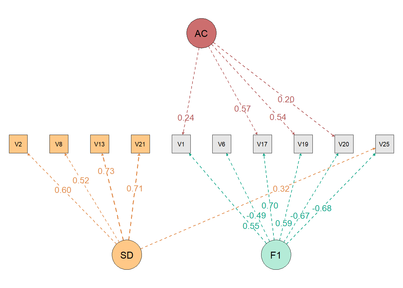



DETAILS OF ANALYSIS

Number of participants                      :   300 
Number of items                             :    10 
Items selected as SD items                  :  1, 2, 3, 4
Items selected as unbalanced                :  0
Dispersion Matrix                           : Polychoric Correlations
Method for factor extraction                : Unweighted Least Squares (ULS)
Rotation Method                             : none

-----------------------------------------------------------------------

Univariate item descriptives

Item       Mean        Variance    Skewness     Kurtosis (Zero centered)

Item   1   3.667       1.260      -0.555       -0.566
Item   2   3.263       1.760      -0.379       -1.005
Item   3   2.317       1.695       0.601       -0.880
Item   4   2.947       1.924      -0.033       -1.284
Item   5   3.643       1.374      -0.565       -0.535
Item   6   2.467       1.802       0.487       -0.967
Item   7   3.710       1.678      -0.652       -0.716
Item   8   3.493       1.629      -0.411       -0.862
Item   9   1.997       1.515       1.041       -0.011
Item  10   1.687       0.925       1.293        0.838

Polychoric correlation is advised when the univariate distributions of ordinal items are
asymmetric or with excess of kurtosis. If both indices are lower than one in absolute value,
then Pearson correlation is advised. You can read more about this subject in:

Muthen, B., & Kaplan D. (1985). A Comparison of Some Methodologies for the Factor Analysis of
Non-Normal Likert Variables. British Journal of Mathematical and Statistical Psychology, 38, 171-189.

Muthen, B., & Kaplan D. (1992). A Comparison of Some Methodologies for the Factor Analysis of
Non-Normal Likert Variables: A Note on the Size of the Model. British Journal of Mathematical
and Statistical Psychology, 45, 19-30. 

-----------------------------------------------------------------------

Adequacy of the dispersion matrix

Determinant of the matrix     = 0.047816437916936
Bartlett's statistic          =   896.4 (df =    45; P = 0.000000)
Kaiser-Meyer-Olkin (KMO) test = 0.76664 (fair)

-----------------------------------------------------------------------
EXPLORATORY FACTOR ANALYSIS CONTROLLING SOCIAL DESIRABILITY AND ACQUIESCENCE
-----------------------------------------------------------------------

Robust Goodness of Fit statistics

          Root Mean Square Error of Approximation (RMSEA) = 0.032

 Robust Mean-Scaled Chi Square with 23 degrees of freedom = 30.146

              Non-Normed Fit Index (NNFI; Tucker & Lewis) = 0.989
                              Comparative Fit Index (CFI) = 0.994
                              Goodness of Fit Index (GFI) = 0.977

-----------------------------------------------------------------------

                  Root Mean Square Residuals (RMSR) = 0.0452
Expected mean value of RMSR for an acceptable model = 0.0578 (Kelley's criterion)

-----------------------------------------------------------------------

Unrotated loading matrix

         Factor SD Factor AC Factor 1
Item   1   0.60254   0.00000  0.00000
Item   2   0.51526   0.00000  0.00000
Item   3   0.72705   0.00000  0.00000
Item   4   0.71128   0.00000  0.00000
Item   5  -0.07850   0.23759  0.54830
Item   6   0.27518   0.00218 -0.49050
Item   7  -0.16412   0.57410  0.70138
Item   8  -0.14319   0.54069  0.59107
Item   9   0.26558   0.19606 -0.66804
Item  10   0.31731   0.06248 -0.68221

This analysis allows controlling the effects of two response biases: Social Desirability and Acquiescence, extracting the variance due to these factors before extracting the content variance. If you don’t have or want to control acquiescence, simply change the argument contAC = TRUE to contAC = FALSE .

We see that Bartlett’s test of sphericity and KMO were calculated before proceeding with Exploratory Factor Analysis. Furthermore, the model fit indices were calculated. We also see that items 6, 9 and 10 have even high loadings on the desirability factor (“Factor SD”), and items 5, 7 and 8 on the acquiescence factor (“Factor AC”).

The cool thing is that it allows you to calculate people’s factor scores. Factor scores work like when you calculate the mean score of an instrument to correlate with others, but calculating mean scores has certain assumptions, while factor scores have others. So, to calculate the factor scores while controlling the SD and acquiescence biases, simply leave the factor scores argument as TRUE (factor_scores = TRUE) and save the result in some variable. In our case, we save the results in the res variable.

To save only the factor scores, simply extract the scores from the list.

factor_scores <- res$Factor_scores

This way, just put this column of factor scores together with your data (using cbind()) and then calculate whatever analysis you want.

8.6.2 Controlling with MIMIC and Quadruples (Bastos & Valentini, 2023)

To run a MIMIC with Quadruples, we first have to install the lavaan (Rosseel, 2012) package to run the analyzes and for database simulation and semplot (Epskamp, 2022) package for visualization.

install.packages("lavaan")
install.packages("semPlot")

And tell the program that we are going to use the functions of these packages.

library(lavaan)
library(semPlot)

Let’s simulate the data with quadruplets for us to use.

#Quadruple Factor Loadings on Social Desirability
FactorLoadingsSDQ<- rep(0.3, 16)*c(1,-1,1,-1)

#Quadruple Factor Loadings on the Target Construct
RandomFactorLoadingsQ<-rep(0.7, 16)*c(-1,-1,1,1)

# Factor Loads of the extra item in the Target Construct
set.seed(2021)
RandomFactorLoadings <- round(runif((10), min = .3, max = .8), 3)

# Desirability Regressions for Target Construct items
set.seed(2021)
RandomSDregression <- round(runif((10), min = .1, max = .5), 3)

# Item Thresholds
set.seed(2020)
thld1Vet<-round(runif(26, min=-2, max=.5),3)
thld2Vet<-round(thld1Vet +.5,3)
thld3Vet<-round(thld1Vet + 1,3)
thld4Vet<-round(thld1Vet + 1.5,3)

# Simulated Model
simModel <- paste0("fator1 =~",RandomFactorLoadings[1],"*it1 +",
                         RandomFactorLoadings[2],"*it2 +",
                         RandomFactorLoadings[3],"*it3 +",
                         RandomFactorLoadings[4],"*it4 +",
                         RandomFactorLoadings[5],"*it5 +",
                         RandomFactorLoadingsQ[1],"*sd1 +",
                         RandomFactorLoadingsQ[2],"*sd2 +",
                         RandomFactorLoadingsQ[3],"*sd3 +",
                         RandomFactorLoadingsQ[4],"*sd4 +",
                         RandomFactorLoadingsQ[5],"*sd5 +",
                         RandomFactorLoadingsQ[6],"*sd6 +",
                         RandomFactorLoadingsQ[7],"*sd7 +",
                         RandomFactorLoadingsQ[8],"*sd8\n",
                             
                         "fator2 =~", RandomFactorLoadingsQ[6],"*it6 +", 
                         RandomFactorLoadingsQ[7],"*it7 +",
                         RandomFactorLoadingsQ[8],"*it8 +",
                         RandomFactorLoadingsQ[9],"*it9 +",
                         RandomFactorLoadingsQ[10],"*it10 +",
                         RandomFactorLoadingsQ[9],"*sd9 +",
                         RandomFactorLoadingsQ[10],"*sd10 +",
                         RandomFactorLoadingsQ[11],"*sd11 +",
                         RandomFactorLoadingsQ[12],"*sd12 +",
                         RandomFactorLoadingsQ[13],"*sd13 +",
                         RandomFactorLoadingsQ[14],"*sd14 +",
                         RandomFactorLoadingsQ[15],"*sd15 +",
                         RandomFactorLoadingsQ[16],"*sd16\n",
                             
                         "SD =~", FactorLoadingsSDQ[1], "*sd1 +", 
                         FactorLoadingsSDQ[2],"*sd2 +",
                         FactorLoadingsSDQ[3],"*sd3 +",
                         FactorLoadingsSDQ[4],"*sd4 +",
                         FactorLoadingsSDQ[5], "*sd5 +",
                         FactorLoadingsSDQ[6],"*sd6 +",
                         FactorLoadingsSDQ[7],"*sd7 +",
                         FactorLoadingsSDQ[8],"*sd8 +",
                         FactorLoadingsSDQ[9], "*sd9 +",
                         FactorLoadingsSDQ[10],"*sd10 +",
                         FactorLoadingsSDQ[11],"*sd11 +",
                         FactorLoadingsSDQ[12],"*sd12 +",
                         FactorLoadingsSDQ[13], "*sd13 +",
                         FactorLoadingsSDQ[14],"*sd14 +",
                         FactorLoadingsSDQ[15],"*sd15 +",
                         FactorLoadingsSDQ[16],"*sd16\n",
                             
                         "SD ~~ 1*SD\n",
                         "fator1 ~~ 1*fator1\n",
                         "fator2 ~~ 1*fator2\n",
                         "fator1 ~~ 0*SD\n",
                         "fator2 ~~ 0*SD\n",
                         "fator1 ~~ .3*fator2\n",
                             
                         "it1 ~",RandomSDregression[1],"*SD\n",
                         "it2 ~",RandomSDregression[2],"*SD\n",
                         "it3 ~",RandomSDregression[3],"*SD\n",
                         "it4 ~",RandomSDregression[4],"*SD\n",
                         "it5 ~",RandomSDregression[5],"*SD\n",
                         "it6 ~",RandomSDregression[6],"*SD\n",
                         "it7 ~",RandomSDregression[7],"*SD\n",
                         "it8 ~",RandomSDregression[8],"*SD\n",
                         "it9 ~",RandomSDregression[9],"*SD\n",
                         "it10 ~",RandomSDregression[10],"*SD\n",
                             
                         "sd1 |",thld1Vet[1],"*t1 +", thld2Vet[1], "*t2 +", 
                         thld3Vet[1],"*t3 +",thld4Vet[1],"*t4\n",
                         "sd2 |",thld1Vet[2],"*t1 +", thld2Vet[2], "*t2 +", 
                         thld3Vet[2],"*t3 +",thld4Vet[2],"*t4\n",
                        "sd3 |",thld1Vet[3],"*t1 +", thld2Vet[3], "*t2 +", 
                        thld3Vet[3],"*t3 +",thld4Vet[3],"*t4\n",
                        "sd4 |",thld1Vet[4],"*t1 +", thld2Vet[4], "*t2 +",
                        thld3Vet[4],"*t3 +",thld4Vet[4],"*t4\n",
                        "it1 |",thld1Vet[5],"*t1 +", thld2Vet[5], "*t2 +",
                        thld3Vet[5],"*t3 +",thld4Vet[5],"*t4\n",
                        "it2 |",thld1Vet[6],"*t1 +", thld2Vet[6], "*t2 +",
                        thld3Vet[6],"*t3 +",thld4Vet[6],"*t4\n",
                        "it3 |",thld1Vet[7],"*t1 +", thld2Vet[7], "*t2 +",
                        thld3Vet[7],"*t3 +",thld4Vet[7],"*t4\n",
                        "it4 |",thld1Vet[8],"*t1 +", thld2Vet[8], "*t2 +",
                        thld3Vet[8],"*t3 +",thld4Vet[8],"*t4\n",
                        "it5 |",thld1Vet[9],"*t1 +", thld2Vet[9], "*t2 +",
                        thld3Vet[9],"*t3 +",thld4Vet[9],"*t4\n",
                        "it6 |",thld1Vet[10],"*t1 +", thld2Vet[10], "*t2 +",
                        thld3Vet[10],"*t3 +",thld4Vet[10],"*t4\n",
                        "it7 |",thld1Vet[11],"*t1 +", thld2Vet[11], "*t2 +",
                        thld3Vet[11],"*t3 +",thld4Vet[11],"*t4\n",
                        "it8 |",thld1Vet[12],"*t1 +", thld2Vet[12], "*t2 +",
                        thld3Vet[12],"*t3 +",thld4Vet[12],"*t4\n",
                        "it9 |",thld1Vet[13],"*t1 +", thld2Vet[13], "*t2 +",
                        thld3Vet[13],"*t3 +",thld4Vet[13],"*t4\n",
                        "it10 |",thld1Vet[14],"*t1 +", thld2Vet[14], "*t2 +",
                        thld3Vet[14],"*t3 +",thld4Vet[14],"*t4\n",
                        "sd5 |",thld1Vet[15],"*t1 +", thld2Vet[15], "*t2 +",
                        thld3Vet[15],"*t3 +",thld4Vet[15],"*t4\n",
                        "sd6 |",thld1Vet[16],"*t1 +", thld2Vet[16], "*t2 +",
                        thld3Vet[16],"*t3 +",thld4Vet[16],"*t4\n",
                        "sd7 |",thld1Vet[17],"*t1 +", thld2Vet[17], "*t2 +",
                        thld3Vet[17],"*t3 +",thld4Vet[17],"*t4\n",
                        "sd8 |",thld1Vet[18],"*t1 +", thld2Vet[18], "*t2 +",
                        thld3Vet[18],"*t3 +",thld4Vet[18],"*t4\n",
                        "sd9 |",thld1Vet[19],"*t1 +", thld2Vet[19], "*t2 +",
                        thld3Vet[19],"*t3 +",thld4Vet[19],"*t4\n",
                        "sd10 |",thld1Vet[20],"*t1 +", thld2Vet[20], "*t2 +",
                        thld3Vet[20],"*t3 +",thld4Vet[20],"*t4\n",
                        "sd11 |",thld1Vet[21],"*t1 +", thld2Vet[21], "*t2 +",
                        thld3Vet[21],"*t3 +",thld4Vet[21],"*t4\n",
                        "sd12 |",thld1Vet[22],"*t1 +", thld2Vet[22], "*t2 +",
                        thld3Vet[22],"*t3 +",thld4Vet[22],"*t4\n",
                        "sd13 |",thld1Vet[23],"*t1 +", thld2Vet[23], "*t2 +",
                        thld3Vet[23],"*t3 +",thld4Vet[23],"*t4\n",
                        "sd14 |",thld1Vet[24],"*t1 +", thld2Vet[24], "*t2 +",
                        thld3Vet[24],"*t3 +",thld4Vet[24],"*t4\n",
                        "sd15 |",thld1Vet[25],"*t1 +", thld2Vet[25], "*t2 +",
                        thld3Vet[25],"*t3 +",thld4Vet[25],"*t4\n",
                        "sd16 |",thld1Vet[26],"*t1 +", thld2Vet[26], "*t2 +",
                        thld3Vet[26],"*t3 +",thld4Vet[26],"*t4")

#Simulating the Data
simulatedData <- lavaan::simulateData(model = simModel,
                                       model.type = "sem",
                                       sample.nobs = 4000,
                                       seed = 2024,
                                       return.type = "data.frame",
                                       standardized = TRUE
                                       )

In the simulated data, we have items from it1 to it10 (which are items that are not made in quadruple format), items sd1 to sd16 (which are items in quadruple format), and are in the 5-point Likert format. See a summary of the items below.

summary(simulatedData)

      it1             it2             it3             it4       
 Min.   :1.000   Min.   :1.000   Min.   :1.000   Min.   :1.000  
 1st Qu.:3.000   1st Qu.:4.000   1st Qu.:4.000   1st Qu.:2.000  
 Median :5.000   Median :5.000   Median :5.000   Median :4.000  
 Mean   :4.146   Mean   :4.311   Mean   :4.163   Mean   :3.381  
 3rd Qu.:5.000   3rd Qu.:5.000   3rd Qu.:5.000   3rd Qu.:5.000  
 Max.   :5.000   Max.   :5.000   Max.   :5.000   Max.   :5.000  
      it5             sd1            sd2             sd3             sd4       
 Min.   :1.000   Min.   :1.00   Min.   :1.000   Min.   :1.000   Min.   :1.000  
 1st Qu.:4.000   1st Qu.:1.00   1st Qu.:2.000   1st Qu.:1.000   1st Qu.:2.000  
 Median :5.000   Median :2.00   Median :4.000   Median :2.000   Median :3.000  
 Mean   :4.445   Mean   :2.52   Mean   :3.353   Mean   :2.585   Mean   :3.092  
 3rd Qu.:5.000   3rd Qu.:4.00   3rd Qu.:5.000   3rd Qu.:4.000   3rd Qu.:4.000  
 Max.   :5.000   Max.   :5.00   Max.   :5.000   Max.   :5.000   Max.   :5.000  
      sd5             sd6             sd7             sd8       
 Min.   :1.000   Min.   :1.000   Min.   :1.000   Min.   :1.000  
 1st Qu.:2.000   1st Qu.:1.000   1st Qu.:1.000   1st Qu.:1.000  
 Median :3.000   Median :3.000   Median :1.000   Median :2.000  
 Mean   :3.314   Mean   :2.846   Mean   :1.655   Mean   :2.485  
 3rd Qu.:5.000   3rd Qu.:4.000   3rd Qu.:2.000   3rd Qu.:4.000  
 Max.   :5.000   Max.   :5.000   Max.   :5.000   Max.   :5.000  
      it6             it7             it8             it9       
 Min.   :1.000   Min.   :1.000   Min.   :1.000   Min.   :1.000  
 1st Qu.:1.000   1st Qu.:1.000   1st Qu.:1.000   1st Qu.:1.000  
 Median :2.000   Median :2.000   Median :2.000   Median :1.000  
 Mean   :2.623   Mean   :2.139   Mean   :2.186   Mean   :1.983  
 3rd Qu.:4.000   3rd Qu.:3.000   3rd Qu.:3.000   3rd Qu.:3.000  
 Max.   :5.000   Max.   :5.000   Max.   :5.000   Max.   :5.000  
      it10            sd9             sd10            sd11      
 Min.   :1.000   Min.   :1.000   Min.   :1.000   Min.   :1.000  
 1st Qu.:2.000   1st Qu.:1.000   1st Qu.:3.000   1st Qu.:3.000  
 Median :3.000   Median :3.000   Median :4.000   Median :4.000  
 Mean   :3.297   Mean   :2.853   Mean   :3.792   Mean   :3.942  
 3rd Qu.:5.000   3rd Qu.:4.000   3rd Qu.:5.000   3rd Qu.:5.000  
 Max.   :5.000   Max.   :5.000   Max.   :5.000   Max.   :5.000  
      sd12            sd13            sd14            sd15      
 Min.   :1.000   Min.   :1.000   Min.   :1.000   Min.   :1.000  
 1st Qu.:4.000   1st Qu.:1.000   1st Qu.:1.000   1st Qu.:1.000  
 Median :5.000   Median :1.000   Median :1.000   Median :1.000  
 Mean   :4.264   Mean   :1.994   Mean   :1.686   Mean   :1.814  
 3rd Qu.:5.000   3rd Qu.:3.000   3rd Qu.:2.000   3rd Qu.:2.000  
 Max.   :5.000   Max.   :5.000   Max.   :5.000   Max.   :5.000  
      sd16      
 Min.   :1.000  
 1st Qu.:3.000  
 Median :5.000  
 Mean   :4.019  
 3rd Qu.:5.000  
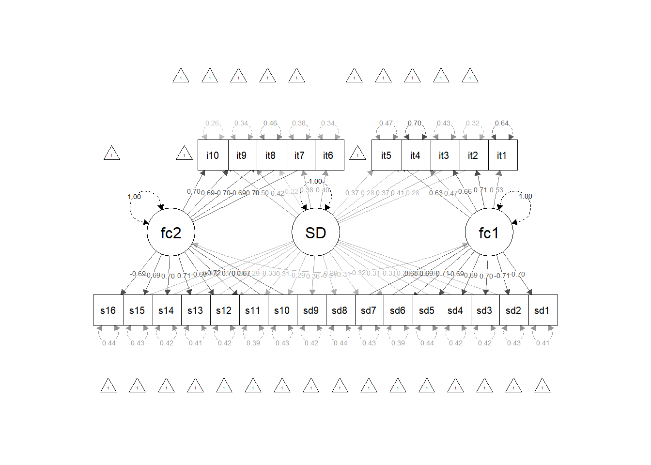
 Max.   :5.000

You will get to understand the model better now, when we configure it. We have 26 items, 4 of which are quadruples (16 items), and 10 items outside the quadruples to try to control social desirability. Let’s configure the model the way you would with your database, that is, we will place all items (quadruples or not) of a given factor to estimate that factor. For example, items it1 to it4 and items sd1 to sd8 are Factor 1 items, so we will estimate Factor 1 with these items. The same logic applies to Factor 2. To estimate desirability, we will only use the quadruples, given that only in the quadruples we manipulated the items to have desirability. We also have to maintain the content factors (Factor 1 and Factor 2) with a correlation equal to 0 with the desirability factor. This is a necessary step to be able to carry out the calculation, otherwise we will have to estimate more parameters than we have information about. Finally, we will perform a desirability regression for the items that were not manipulated in quadruples, to control for the desirability of these extra items.

empiricalModel <- "
              factor1 =~ NA*it1 + it2 + it3 + it4 + it5 + sd1 + sd2 + sd3 + 
              sd4 + sd5 + sd6 + sd7 + sd8

              factor2 =~ NA*it6 + it7 + it8 + it9 + it10 + sd9 + sd10 + sd11 + 
              sd12 + sd13 + sd14 + sd15 + sd16
              
              SD =~ NA*sd1 + sd2 + sd3 + sd4 + sd5 + sd6 + sd7 + sd8 + sd9 +
              sd10 + sd11 + sd12 + sd13 + sd14 + sd15 + sd16
              
              SD ~~ 1*SD
              factor1 ~~ 1*factor1
              factor2 ~~ 1*factor2

              factor1 ~~ 0*SD
              factor2 ~~ 0*SD
              factor1 ~~ factor2
              
              it1 ~ SD
              it2 ~ SD
              it3 ~ SD
              it4 ~ SD
              it5 ~ SD
              it6 ~ SD
              it7 ~ SD
              it8 ~ SD
              it9 ~ SD
              it10 ~SD"

E agora, rodaremos a análise da seguinte forma. Como temos itens ordinais, falamos para o programa que os itens são ordinais e usamos o estimador “WLSMV”.

sem.fit <- sem(model = empiricalModel,
               data = simulatedData,
               estimator = "WLSMV",
               ordered = TRUE
               ) 

summary(sem.fit, 
        standardized=TRUE,
        fit.measures = TRUE
        )

lavaan 0.6-19 ended normally after 39 iterations

  Estimator                                       DWLS
  Optimization method                           NLMINB
  Number of model parameters                       157

  Number of observations                          4000

Model Test User Model:
                                              Standard      Scaled
  Test Statistic                               134.500     262.032
  Degrees of freedom                               272         272
  P-value (Chi-square)                           1.000       0.657
  Scaling correction factor                                  0.828
  Shift parameter                                           99.666
    simple second-order correction                                

Model Test Baseline Model:

  Test statistic                            182093.691   68350.757
  Degrees of freedom                               325         325
  P-value                                        0.000       0.000
  Scaling correction factor                                  2.672

User Model versus Baseline Model:

  Comparative Fit Index (CFI)                    1.000       1.000
  Tucker-Lewis Index (TLI)                       1.001       1.000
                                                                  
  Robust Comparative Fit Index (CFI)                         1.000
  Robust Tucker-Lewis Index (TLI)                            1.000

Root Mean Square Error of Approximation:

  RMSEA                                          0.000       0.000
  90 Percent confidence interval - lower         0.000       0.000
  90 Percent confidence interval - upper         0.000       0.005
  P-value H_0: RMSEA <= 0.050                    1.000       1.000
  P-value H_0: RMSEA >= 0.080                    0.000       0.000
                                                                  
  Robust RMSEA                                               0.001
  90 Percent confidence interval - lower                     0.000
  90 Percent confidence interval - upper                     0.010
  P-value H_0: Robust RMSEA <= 0.050                         1.000
  P-value H_0: Robust RMSEA >= 0.080                         0.000

Standardized Root Mean Square Residual:

  SRMR                                           0.011       0.011

Parameter Estimates:

  Parameterization                               Delta
  Standard errors                           Robust.sem
  Information                                 Expected
  Information saturated (h1) model        Unstructured

Latent Variables:
                   Estimate  Std.Err  z-value  P(>|z|)   Std.lv  Std.all
  factor1 =~                                                            
    it1               0.533    0.015   34.800    0.000    0.533    0.533
    it2               0.713    0.013   54.803    0.000    0.713    0.713
    it3               0.657    0.013   49.768    0.000    0.657    0.657
    it4               0.468    0.015   31.011    0.000    0.468    0.468
    it5               0.631    0.015   42.576    0.000    0.631    0.631
    sd1              -0.700    0.011  -63.228    0.000   -0.700   -0.700
    sd2              -0.710    0.011  -66.102    0.000   -0.710   -0.710
    sd3               0.701    0.011   64.861    0.000    0.701    0.701
    sd4               0.694    0.011   62.012    0.000    0.694    0.694
    sd5              -0.687    0.011  -60.382    0.000   -0.687   -0.687
    sd6              -0.710    0.011  -66.615    0.000   -0.710   -0.710
    sd7               0.690    0.013   52.042    0.000    0.690    0.690
    sd8               0.683    0.012   58.091    0.000    0.683    0.683
  factor2 =~                                                            
    it6               0.705    0.011   64.358    0.000    0.705    0.705
    it7              -0.692    0.012  -57.695    0.000   -0.692   -0.692
    it8              -0.701    0.011  -62.954    0.000   -0.701   -0.701
    it9               0.690    0.012   55.503    0.000    0.690    0.690
    it10              0.702    0.012   59.851    0.000    0.702    0.702
    sd9               0.673    0.011   59.095    0.000    0.673    0.673
    sd10              0.698    0.011   61.611    0.000    0.698    0.698
    sd11             -0.719    0.012  -62.245    0.000   -0.719   -0.719
    sd12             -0.687    0.013  -54.227    0.000   -0.687   -0.687
    sd13              0.707    0.011   61.651    0.000    0.707    0.707
    sd14              0.703    0.013   55.083    0.000    0.703    0.703
    sd15             -0.692    0.013  -54.861    0.000   -0.692   -0.692
    sd16             -0.687    0.012  -58.792    0.000   -0.687   -0.687
  SD =~                                                                 
    sd1               0.315    0.019   16.764    0.000    0.315    0.315
    sd2              -0.261    0.019  -13.479    0.000   -0.261   -0.261
    sd3               0.293    0.019   15.763    0.000    0.293    0.293
    sd4              -0.307    0.019  -16.490    0.000   -0.307   -0.307
    sd5               0.305    0.019   15.992    0.000    0.305    0.305
    sd6              -0.318    0.018  -17.535    0.000   -0.318   -0.318
    sd7               0.311    0.021   14.856    0.000    0.311    0.311
    sd8              -0.308    0.019  -16.326    0.000   -0.308   -0.308
    sd9               0.358    0.018   19.441    0.000    0.358    0.358
    sd10             -0.292    0.020  -14.596    0.000   -0.292   -0.292
    sd11              0.309    0.020   15.431    0.000    0.309    0.309
    sd12             -0.326    0.020  -16.032    0.000   -0.326   -0.326
    sd13              0.292    0.020   14.543    0.000    0.292    0.292
    sd14             -0.300    0.021  -14.325    0.000   -0.300   -0.300
    sd15              0.308    0.021   14.940    0.000    0.308    0.308
    sd16             -0.297    0.020  -14.918    0.000   -0.297   -0.297

Regressions:
                   Estimate  Std.Err  z-value  P(>|z|)   Std.lv  Std.all
  it1 ~                                                                 
    SD                0.280    0.020   14.105    0.000    0.280    0.280
  it2 ~                                                                 
    SD                0.413    0.020   20.933    0.000    0.413    0.413
  it3 ~                                                                 
    SD                0.369    0.020   18.801    0.000    0.369    0.369
  it4 ~                                                                 
    SD                0.280    0.019   15.057    0.000    0.280    0.280
  it5 ~                                                                 
    SD                0.366    0.020   18.017    0.000    0.366    0.366
  it6 ~                                                                 
    SD                0.400    0.018   21.915    0.000    0.400    0.400
  it7 ~                                                                 
    SD                0.382    0.019   19.789    0.000    0.382    0.382
  it8 ~                                                                 
    SD                0.215    0.020   10.530    0.000    0.215    0.215
  it9 ~                                                                 
    SD                0.424    0.019   22.454    0.000    0.424    0.424
  it10 ~                                                                
    SD                0.496    0.017   29.103    0.000    0.496    0.496

Covariances:
                   Estimate  Std.Err  z-value  P(>|z|)   Std.lv  Std.all
  factor1 ~~                                                            
    SD                0.000                               0.000    0.000
  factor2 ~~                                                            
    SD                0.000                               0.000    0.000
  factor1 ~~                                                            
    factor2          -0.290    0.017  -17.440    0.000   -0.290   -0.290

Thresholds:
                   Estimate  Std.Err  z-value  P(>|z|)   Std.lv  Std.all
    it1|t1           -1.657    0.034  -49.184    0.000   -1.657   -1.657
    it1|t2           -1.146    0.025  -45.186    0.000   -1.146   -1.146
    it1|t3           -0.670    0.022  -31.120    0.000   -0.670   -0.670
    it1|t4           -0.182    0.020   -9.133    0.000   -0.182   -0.182
    it2|t1           -1.793    0.037  -48.349    0.000   -1.793   -1.793
    it2|t2           -1.332    0.028  -48.013    0.000   -1.332   -1.332
    it2|t3           -0.834    0.023  -36.989    0.000   -0.834   -0.834
    it2|t4           -0.361    0.020  -17.793    0.000   -0.361   -0.361
    it3|t1           -1.680    0.034  -49.095    0.000   -1.680   -1.680
    it3|t2           -1.161    0.026  -45.489    0.000   -1.161   -1.161
    it3|t3           -0.700    0.022  -32.270    0.000   -0.700   -0.700
    it3|t4           -0.188    0.020   -9.417    0.000   -0.188   -0.188
    it4|t1           -1.012    0.024  -42.192    0.000   -1.012   -1.012
    it4|t2           -0.537    0.021  -25.718    0.000   -0.537   -0.537
    it4|t3           -0.029    0.020   -1.486    0.137   -0.029   -0.029
    it4|t4            0.468    0.021   22.674    0.000    0.468    0.468
    it5|t1           -1.991    0.043  -45.939    0.000   -1.991   -1.991
    it5|t2           -1.504    0.031  -49.218    0.000   -1.504   -1.504
    it5|t3           -1.006    0.024  -42.032    0.000   -1.006   -1.006
    it5|t4           -0.501    0.021  -24.136    0.000   -0.501   -0.501
    sd1|t1           -0.393    0.020  -19.267    0.000   -0.393   -0.393
    sd1|t2            0.106    0.020    5.343    0.000    0.106    0.106
    sd1|t3            0.608    0.021   28.678    0.000    0.608    0.608
    sd1|t4            1.088    0.025   43.998    0.000    1.088    1.088
    sd2|t1           -1.004    0.024  -41.979    0.000   -1.004   -1.004
    sd2|t2           -0.482    0.021  -23.297    0.000   -0.482   -0.482
    sd2|t3           -0.024    0.020   -1.233    0.218   -0.024   -0.024
    sd2|t4            0.478    0.021   23.110    0.000    0.478    0.478
    sd3|t1           -0.436    0.021  -21.270    0.000   -0.436   -0.436
    sd3|t2            0.051    0.020    2.561    0.010    0.051    0.051
    sd3|t3            0.550    0.021   26.244    0.000    0.550    0.550
    sd3|t4            1.057    0.024   43.289    0.000    1.057    1.057
    sd4|t1           -0.812    0.022  -36.260    0.000   -0.812   -0.812
    sd4|t2           -0.331    0.020  -16.380    0.000   -0.331   -0.331
    sd4|t3            0.174    0.020    8.754    0.000    0.174    0.174
    sd4|t4            0.705    0.022   32.451    0.000    0.705    0.705
    sd5|t1           -0.979    0.024  -41.332    0.000   -0.979   -0.979
    sd5|t2           -0.468    0.021  -22.705    0.000   -0.468   -0.468
    sd5|t3            0.029    0.020    1.486    0.137    0.029    0.029
    sd5|t4            0.497    0.021   23.981    0.000    0.497    0.497
    sd6|t1           -0.643    0.021  -30.055    0.000   -0.643   -0.643
    sd6|t2           -0.124    0.020   -6.227    0.000   -0.124   -0.124
    sd6|t3            0.358    0.020   17.636    0.000    0.358    0.358
    sd6|t4            0.853    0.023   37.626    0.000    0.853    0.853
    sd7|t1            0.385    0.020   18.922    0.000    0.385    0.385
    sd7|t2            0.873    0.023   38.259    0.000    0.873    0.873
    sd7|t3            1.395    0.029   48.613    0.000    1.395    1.395
    sd7|t4            1.842    0.038   47.877    0.000    1.842    1.842
    sd8|t1           -0.374    0.020  -18.389    0.000   -0.374   -0.374
    sd8|t2            0.135    0.020    6.765    0.000    0.135    0.135
    sd8|t3            0.633    0.021   29.688    0.000    0.633    0.633
    sd8|t4            1.129    0.025   44.854    0.000    1.129    1.129
    it6|t1           -0.466    0.021  -22.611    0.000   -0.466   -0.466
    it6|t2            0.036    0.020    1.834    0.067    0.036    0.036
    it6|t3            0.517    0.021   24.851    0.000    0.517    0.517
    it6|t4            1.015    0.024   42.271    0.000    1.015    1.015
    it7|t1           -0.077    0.020   -3.857    0.000   -0.077   -0.077
    it7|t2            0.413    0.020   20.206    0.000    0.413    0.413
    it7|t3            0.884    0.023   38.602    0.000    0.884    0.884
    it7|t4            1.402    0.029   48.665    0.000    1.402    1.402
    it8|t1           -0.140    0.020   -7.049    0.000   -0.140   -0.140
    it8|t2            0.358    0.020   17.636    0.000    0.358    0.358
    it8|t3            0.881    0.023   38.488    0.000    0.881    0.881
    it8|t4            1.398    0.029   48.639    0.000    1.398    1.398
    it9|t1            0.039    0.020    1.960    0.050    0.039    0.039
    it9|t2            0.540    0.021   25.842    0.000    0.540    0.540
    it9|t3            1.049    0.024   43.108    0.000    1.049    1.049
    it9|t4            1.583    0.032   49.325    0.000    1.583    1.583
    it10|t1          -0.950    0.023  -40.539    0.000   -0.950   -0.950
    it10|t2          -0.467    0.021  -22.643    0.000   -0.467   -0.467
    it10|t3           0.023    0.020    1.138    0.255    0.023    0.023
    it10|t4           0.532    0.021   25.502    0.000    0.532    0.532
    sd9|t1           -0.666    0.022  -30.968    0.000   -0.666   -0.666
    sd9|t2           -0.136    0.020   -6.859    0.000   -0.136   -0.136
    sd9|t3            0.352    0.020   17.385    0.000    0.352    0.352
    sd9|t4            0.882    0.023   38.516    0.000    0.882    0.882
    sd10|t1          -1.352    0.028  -48.222    0.000   -1.352   -1.352
    sd10|t2          -0.857    0.023  -37.742    0.000   -0.857   -0.857
    sd10|t3          -0.344    0.020  -17.008    0.000   -0.344   -0.344
    sd10|t4           0.148    0.020    7.460    0.000    0.148    0.148
    sd11|t1          -1.447    0.030  -48.965    0.000   -1.447   -1.447
    sd11|t2          -0.969    0.024  -41.060    0.000   -0.969   -0.969
    sd11|t3          -0.475    0.021  -22.985    0.000   -0.475   -0.475
    sd11|t4           0.001    0.020    0.032    0.975    0.001    0.001
    sd12|t1          -1.852    0.039  -47.766    0.000   -1.852   -1.852
    sd12|t2          -1.300    0.027  -47.649    0.000   -1.300   -1.300
    sd12|t3          -0.777    0.022  -35.081    0.000   -0.777   -0.777
    sd12|t4          -0.282    0.020  -14.021    0.000   -0.282   -0.282
    sd13|t1           0.043    0.020    2.182    0.029    0.043    0.043
    sd13|t2           0.524    0.021   25.130    0.000    0.524    0.524
    sd13|t3           1.032    0.024   42.693    0.000    1.032    1.032
    sd13|t4           1.553    0.031   49.315    0.000    1.553    1.553
    sd14|t1           0.344    0.020   17.008    0.000    0.344    0.344
    sd14|t2           0.852    0.023   37.598    0.000    0.852    0.852
    sd14|t3           1.344    0.028   48.143    0.000    1.344    1.344
    sd14|t4           1.822    0.038   48.081    0.000    1.822    1.822
    sd15|t1           0.203    0.020   10.175    0.000    0.203    0.203
    sd15|t2           0.716    0.022   32.873    0.000    0.716    0.716
    sd15|t3           1.195    0.026   46.097    0.000    1.195    1.195
    sd15|t4           1.728    0.035   48.838    0.000    1.728    1.728
    sd16|t1          -1.570    0.032  -49.325    0.000   -1.570   -1.570
    sd16|t2          -1.053    0.024  -43.186    0.000   -1.053   -1.053
    sd16|t3          -0.548    0.021  -26.183    0.000   -0.548   -0.548
    sd16|t4          -0.039    0.020   -1.960    0.050   -0.039   -0.039

Variances:
                   Estimate  Std.Err  z-value  P(>|z|)   Std.lv  Std.all
    SD                1.000                               1.000    1.000
    factor1           1.000                               1.000    1.000
    factor2           1.000                               1.000    1.000
   .it1               0.637                               0.637    0.637
   .it2               0.322                               0.322    0.322
   .it3               0.432                               0.432    0.432
   .it4               0.703                               0.703    0.703
   .it5               0.468                               0.468    0.468
   .sd1               0.411                               0.411    0.411
   .sd2               0.427                               0.427    0.427
   .sd3               0.423                               0.423    0.423
   .sd4               0.424                               0.424    0.424
   .sd5               0.436                               0.436    0.436
   .sd6               0.395                               0.395    0.395
   .sd7               0.427                               0.427    0.427
   .sd8               0.438                               0.438    0.438
   .it6               0.344                               0.344    0.344
   .it7               0.375                               0.375    0.375
   .it8               0.462                               0.462    0.462
   .it9               0.344                               0.344    0.344
   .it10              0.262                               0.262    0.262
   .sd9               0.419                               0.419    0.419
   .sd10              0.428                               0.428    0.428
   .sd11              0.387                               0.387    0.387
   .sd12              0.422                               0.422    0.422
   .sd13              0.415                               0.415    0.415
   .sd14              0.416                               0.416    0.416
   .sd15              0.425                               0.425    0.425
   .sd16              0.439                               0.439    0.439

We see that the fit index was adequate, all factor loadings were significant and all desirability regressions for the extra items were significant.

To extract factor scores to use for other analyses, simply use the following code.

data_with_scores <- lavPredict(sem.fit,
                                type = "lv",
                                method = "EBM",
                                label = TRUE,
                                append.data = TRUE,
                                optim.method = "bfgs"
                                )

We see that in the variable data_with_scores, the factor scores of each subject were calculated and these scores were added to their database.

Let’s see an image representation of the model using the code below.

semPlot::semPaths(object = sem.fit,
                  layout = "tree2",
                  rotation = 3,
                  whatLabels = "std",
                  edge.label.cex = 0.5,
                  what = "std",
                  edge.color = "black")

8.7 References

Bastos, R. V. S., Valentini, F. (2023). Simulations for two theoretically sound controls for social desirability: MIMIC and Forced-Choice. (Publication No. 157.932 B33s). Master’s thesis, Universidade São Francisco.

Connelly, B. S., & Chang, L. (2016). A meta‐analytic multitrait multirater separation of substance and style in social desirability scales. Journal of Personality, 84(3), 319-334. https://doi.org/10.1111/jopy.12161

Edwards, A. L. (1953). The relationship between the judged desirability of a trait and the probability that the trait will be endorsed. Journal of Applied Psychology, 37(2), 90. https://doi.org/10.1037/h0058073

Edwards, A. L. (1957). The social desirability variable in personality assessment and research. Dryden Press.

Edwards, A. L. (1967). The social desirability variable: A broad statement. In I. A. Berg (Ed.), Response set in personality assessment (pp. 32–47). Aldine.

Epskamp S (2022). semPlot: Path Diagrams and Visual Analysis of Various SEM Packages’ Output. R package. https://CRAN.R-project.org/package=semPlot

Ferrando, P. J. (2005). Factor analytic procedures for assessing social desirability in binary items. Multivariate Behavioral Research, 40(3), 331-349. https://doi.org/10.1207/s15327906mbr4003_3

Ferrando, P. J., Lorenzo-Seva, U., & Chico, E. (2009). A general factor-analytic procedure for assessing response bias in questionnaire measures. Structural Equation Modeling: A Multidisciplinary Journal, 16(2), 364-381. https://doi.org/10.1080/10705510902751374

Graziano, W. G., & Tobin, R. M. (2002). Agreeableness: Dimension of personality or social desirability artifact?. Journal of Personality, 70(5), 695-728. https://doi.org/10.1111/1467-6494.05021

Greenblatt, R. L., Mozdzierz, G. J., & Murphy, T. J. (1984). Content and response‐style in the construct validation of self-report inventories: A canonical analysis. Journal of clinical psychology, 40(6), 1414-1420. https://doi.org/10.1002/1097-4679(198411)40:6\<1414::AID-JCLP2270400624\3.0.CO;2-K>

Griffith, R., Malm, T., English, A., Yoshita, Y., & Gujar, A. (2006). Applicant faking behavior: Teasing apart the influence of situational variance, cognitive biases, and individual differences. In R. L. Griffith & M. H. Peterson (Eds.), A closer examination of applicant faking behavior (pp. 151 – 178). Information Age.

Hebert, J. R., Ma, Y., Clemow, L., Ockene, I. S., Saperia, G., Stanek, E. J., Merriam, P. A., & Ockene, J. K. (1997). Gender differences in social desirability and social approval bias in dietary self-report. American Journal of Epidemiology, 146(12), 1046–1055. https://doi.org/10.1093/oxfordjournals.aje.a009233

King, M. F., & Bruner, G. C. (2000). Social desirability bias: A neglected aspect of validity testing. Psychology & Marketing, 17(2), 79-103. https://doi.org/10.1002/(SICI)1520-6793(200002)17:2<79::AID-MAR2>3.0.CO;2-0

Lange, F., & Dewitte, S. (2019). Measuring pro-environmental behavior: Review and recommendations. Journal of Environmental Psychology, 63, 92-100. https://doi.org/10.1016/j.jenvp.2019.04.009

Lanz, L., Thielmann, I., & Gerpott, F. H. (2022). Are social desirability scales desirable? A meta‐analytic test of the validity of social desirability scales in the context of prosocial behavior. Journal of Personality, 90(2), 203-221. https://doi.org/10.1111/jopy.12662

Leite, W. L., & Cooper, L. A. (2009). Detecting social desirability bias using factor mixture models. Multivariate Behavioral Research, 45(2), 271–293. https://doi.org/10.1080/00273171003680245

Li, A., & Bagger, J. (2006). Using the BIDR to distinguish the effects of impression management and self‐deception on the criterion validity of personality measures: A meta‐analysis. International Journal of Selection and Assessment, 14(2), 131-141. https://doi.org/10.1111/j.1468-2389.2006.00339.x

Malhotra, N. K. (1988). Some observations on the state of the art in marketing research. Journal of the Academy of Marketing Science, 16(1), 4-24. https://doi.org/10.1177/009207038801600102

McFarland, L. A., & Ryan, A. M. (2000). Variance in faking across noncognitive measures. Journal of Applied Psychology, 85(5), 812-821. https://doi.org/10.1037/0021-9010.85.5.812

Mirowsky, J., & Ross, C. E. (1991). Eliminating Defense and Agreement Bias from Measures of the Sense of Control: A 2 X 2 Index. Social Psychology Quarterly, 54(2), 127. https://doi.org/10.2307/2786931

Navarro-Gonzalez D, Vigil-Colet A, Ferrando PJ, Lorenzo-Seva U, Tendeiro JN (2021). vampyr: Factor Analysis Controlling the Effects of Response Bias. https://CRAN.R-project.org/package=vampyr

Nederhof, A. J. (1985). Methods of coping with social desirability bias: A review. European Journal of Social Psychology, 15, 263–280. https://doi.org/10.1002/ejsp.2420150303

Ones, D. S., Viswesvaran, C., & Reiss, A. D. (1996). Role of social desirability in personality testing for personnel selection: The red herring. Journal of applied psychology, 81(6), 660. https://doi.org/10.1037/0021-9010.81.6.660

Paulhus, D. L. (1981). Control of social desirability in personality inventories: Principal-factor deletion. Journal of Research in Personality, 15(3), 383–388. https://doi.org/10.1016/0092-6566(81)90035-0

Paulhus, D. L. (1984). Two-component models of socially desirable responding. Journal of Personality and Social Psychology, 46(3), 598–609. https://doi.org/10.1037/0022-3514.46.3.598

Paulhus, D. L. (1991). Measurement and control of response bias. In J. P. Robinson, P. R. Shaver, & L. S. Wrightsman (Eds.), Measures of social psychological attitudes: Vol. 1. Measures of personality and social psychological attitudes (pp. 17–59). Academic Press. https://doi.org/10.1016/B978-0-12-590241-0.50006-X

Paulhus, D. L., & John, O. P. (1998). Egoistic and moralistic biases in self-perception: The interplay of self-deceptive styles with basic traits and motives. Journal of Personality, 66(6), 1025–1060. https://doi.org/10.1111/1467-6494.00041

Peabody, D. (1967). Trait inferences: Evaluative and descriptive aspects. Journal of Personality and Social Psychology, 7(4, Pt.2), 1-18. https://doi.org/10.1037/h0025230

Peterson, R. A., & Kerin, R. A. (1981). The quality of self-report data: review and synthesis. Review of marketing, 5-20.

Pettersson, E., Mendle, J., Turkheimer, E., Horn, E. E., Ford, D. C., Simms, L. J., & Clark, L. A. (2014). Do maladaptive behaviors exist at one or both ends of personality traits? Psychological Assessment, 26(2), 433-446. https://doi.org/10.1037/a0035587

Pettersson, E., Turkheimer, E., Horn, E. E., & Menatti, A. R. (2012). The General Factor of Personality and Evaluation. European Journal of Personality, 26(3), 292-302. https://doi.org/10.1002/per.839

Podsakoff, P. M., MacKenzie, S. B., Lee, J. Y., & Podsakoff, N. P. (2003). Common method biases in behavioral research: A critical review of the literature and recommended remedies. Journal of Applied Psychology, 88(5), 879-903. https://doi.org/10.1037/0021-9010.88.5.879

R Core Team (2024). R: A Language and Environment for Statistical Computing. R Foundation for Statistical Computing, Vienna, Austria. https://www.R-project.org/

Raymark, P. H., & Tafero, T. L. (2009). Individual differences in the ability to fake on personality measures. Human Performance, 22(1), 86–103. https://doi.org/10.1080/08959280802541039

Riggio, R. E., Salinas, C., & Tucker, J. (1988). Personality and deception ability. Personality and Individual Differences, 9(1), 189–191. https://doi.org/10.1016/0191-8869(88)90050-5

Rosseel, Y. (2012). lavaan: An R Package for Structural Equation Modeling. Journal of Statistical Software, 48(2), 1-36. https://doi.org/10.18637/jss.v048.i02

Saucier, G., Ostendorf, F., & Peabody, D. (2001). The non-evaluative circumplex of personality adjectives. Journal of Personality, 69(4), 537-582. https://doi.org/10.1111/1467-6494.694155

Snell, A. F., Sydell, E. J., & Lueke, S. B. (1999). Towards a theory of applicant faking: Integrating studies of deception. Human Resource Management Review, 9(2), 219–242. https://doi.org/10.1016/S1053-4822(99)00019-4

Ten Berge, J. M. F., & Kiers, H. A. L. (1991). A numerical approach to the approximate and the exact minimum rank of a covariance matrix. Psychometrika, 56, 309–315. https://doi.org/10.1007/BF02294464

Tourangeau, R., & Yan, T. (2007). Sensitive questions in surveys. Psychological Bulletin, 133(5), 859–883. https://doi.org/10.1037/0033-2909.133.5.859

Uziel, L. (2010). Rethinking social desirability scales: From impression management to interpersonally oriented self-control. Perspectives on Psychological Science, 5(3), 243–262. https://doi.org/10.1177/1745691610369465

Vecina, M. L., Chacón, F., & Pérez-Viejo, J. M. (2016). Moral absolutism, self-deception, and moral self-concept in men who commit intimate partner violence: A comparative study with an opposite sample. Violence Against Women, 22(1), 3–16. https://doi.org/10.1177/1077801215597791

de Vries, R. E., Zettler, I., & Hilbig, B. E. (2014). Rethinking trait conceptions of social desirability scales: Impression management as an expression of honesty-humility. Assessment, 21(3), 286–299. https://doi.org/10.1177/1073191113504619

Williams, E. A., Pillai, R., Lowe, K. B., Jung, D., & Herst, D. (2009). Crisis, charisma, values, and voting behavior in the 2004 presidential election. The Leadership Quarterly, 20(2), 70–86. https://doi.org/10.1016/j.leaqua.2009.01.002

Zickar, M. J., & Robie, C. (1999). Modeling faking good on personality items: An item-level analysis. Journal of Applied Psychology, 84(4), 551. https://doi.org/10.1037/0021-9010.84.4.551

Ziegler, M., & Buehner, M. (2009). Modeling socially desirable responding and its effects. Educational and Psychological Measurement, 69(4), 548-565. https://doi.org/10.1177/0013164408324469

Ziegler, M., Maccann, C., & Roberts, R. D. (2011). New perspectives on faking in personality assessment. Oxford University Press.